HTML document: Layout

1 YAML

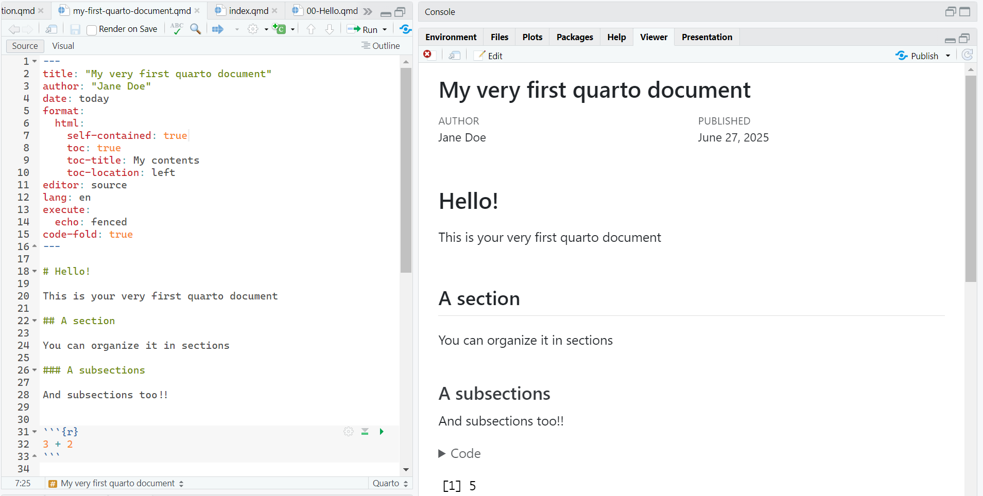
The overall appearance and behavior of the document is specified in the YAML.

Importantly the YAML defines the extension of the file rendering:

HTML default YAML

---
title: "Untitled"
format: html
editor: visual
---

PDF default YAML

---
title: "Untitled"
format: pdf
editor: visual
---

1.1 `editor`

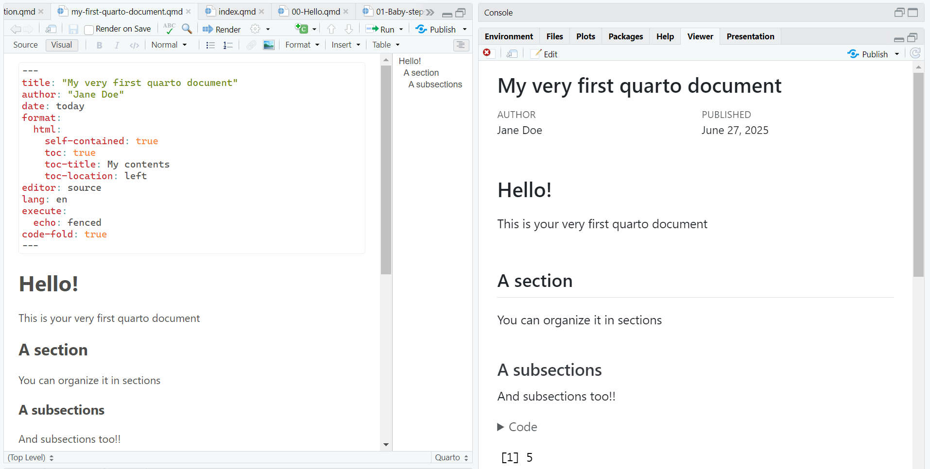
Quarto (as well as as RMarkdown) allows for visualizing the text editor as a WYSIWYG text editor:

1.2 `editor: source`

1.3 `editor: visual`

Warning

Although at the very beginning, the use of the visual editor might be tempting, don’t indulge! Using the source editor is an investment in your future programming skills :)

1.4 `toc`

Table Of Contents: Defines the index of your document and its associated characteristics (e.g., where it is located):

---
title: "My quarto file"
author: "Jane Doe"
date: today
format: 
  html:
    toc: true                
    toc-title: My contents   
    toc-location: left       
---

Be mindful of the indentation!! With the wrong indentation, the YAML breaks down and the document will not compile.

toc: true: Set the table of contents
toc-title: My contents: Define the title of the toc
toc-location: left: Define the position of the toc (options: left, right, body)

1.5 Themes

The default theme of the document can be modified with the predefined themes

---
title: "My quarto file"
author: "Jane Doe"
date: today
format: 
  html:
    toc: true                   
    toc-title: My contents   
    toc-location: left
    theme: superhero  
    fontsize: 32px    
lang: it                     
---

The theme can be defined with the theme: specific_theme in the YAML. Further customization can be brought with other YAML arguments (e.g.,fontsize) or with specific css settings

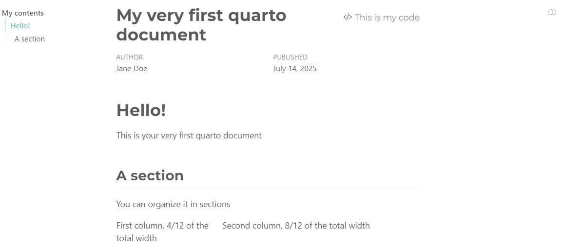
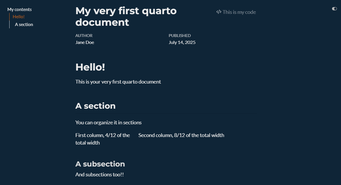
The theme can adapt to specific settings, such as whether you want both ligth and dark theme:

---
format: 
  html:
    theme:
     light: minty
     dark: superhero
---

1.6 Day

1.7 Night

1.8 `lang`

Set the language for your document. This is not the autocorrect!

It sets the language to be used in the cross-referencing of your document (see Section 4).

Language	Code
English	`en`
Chinese	`zh`
Spanish	`es`
French	`fr`
Japanese	`ja`
German	`de`

Language	Code
Portuguese	`pt`
Russian	`ru`
Czech	`cs`
Finnish	`fi`
Dutch	`nl`
Italian	`it`
Polish	`pl`
Korean	`ko`

The YAML is also used to define the references for a document (e.g., the bibliography external file, the references style and so on). See Section 2.6.

1.9 General Layout

Figure 1 illustrates the default setting of an HTML page.

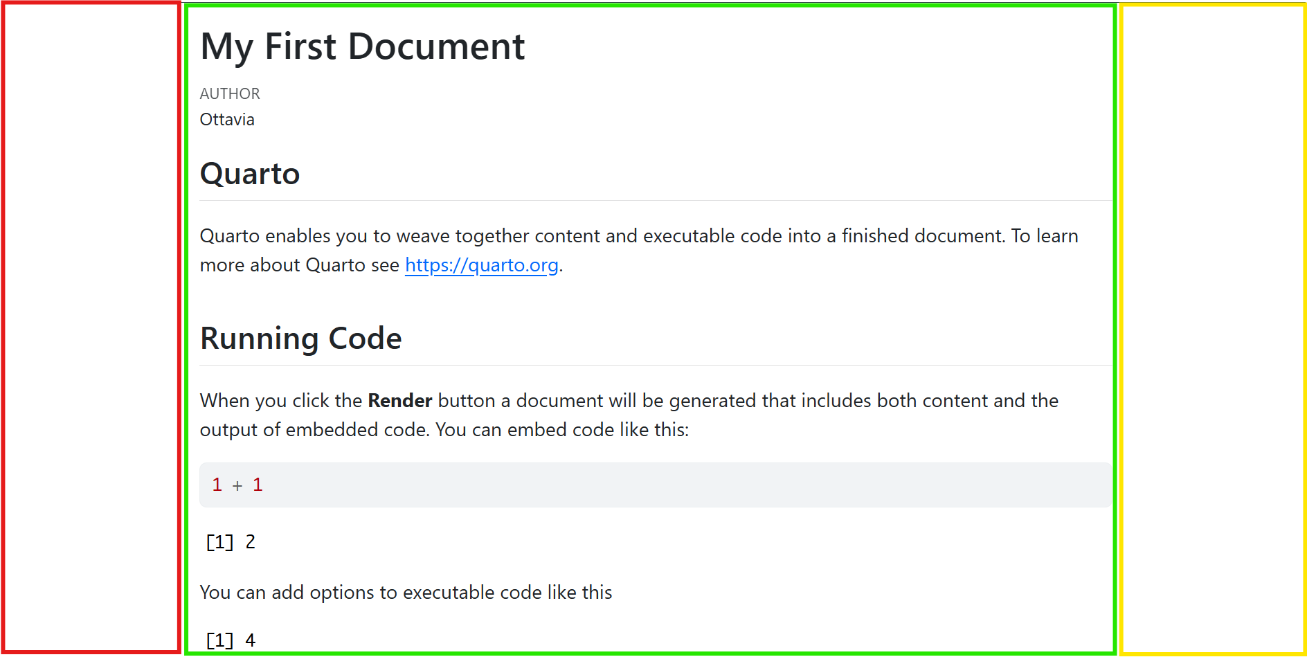
Figure 1: Default layout of an HTML document

The layout is divided into three main parts:

the sidebar on the left side (red rectangle in Figure 1)
the body in the center (green rectangle in Figure 1)
the margin on the right side (yellow rectangle in Figure 1)

Between each of these parts, there is the so-called gutter (i.e., the empty space between the main parts). Its width can be modified as well in the YAML, with default values as follows:

format:
  html: 
    grid:
      sidebar-width: 300px
      body-width: 900px
      margin-width: 300px
      gutter-width: 1.5rem

These settings will affect the entire document. Section 3 presents the layout settings for specific part of the document.

2 Markdown formatting

2.1 Headings

The number of # defines the level of the headings (the lower the number of #, the higher the level)

# First level (H1)

Section

## Second level (H2)

Subsection

### Third level (H3)

Sub-subsection

#### Fourth level (H4)

Paragraph

##### Fifth level (H5)

I frankly have never used that

##### Sixth level (H6)

I have no idea

2.2 Text Formatting

The text formatting is defined through specific tags:

2.2.1 Formatting

*italics*, **bold**, ***bold italics***

italics, bold, bold italics

2.2.2 Super/sub script

textsuperscript^2^, textunderscript~2~

textsuperscript², textunderscript₂

2.2.3 In line code

`this is myinline code`

this is myinline code

Code chunk

There will be a specific lesson on the code chunks

2.3 Links and images

<https://github.com/>

https://github.com/

My link is [here](https://github.com/)

My link is here

![This is an image](img/picture.jpg)

Links & index.qmd

As seen in the GitHub lesson, the index.qmd works as the landing page of a potential website. To include other documents and hyperlink them in the main landing page, we use the syntax for the links (see Section 5).

2.4 Lists

* Main Unordered List
  + First sub-item
  + Second sub-item 
    - It's getting weird

Main Unordered List
- First sub-item
- Second sub-item
  - It’s getting weird

1. Main ordered list
2. Second item
   i) First sub-item 1
      A.  First sub-sub-item 1

Main ordered list
Second item
1. First sub-item 1
  1. First sub-sub-item 1

- [ ] First things first 1
- [ ] Second things second 2

First things first 1
Second things second 2

2.5 Math

In-line math:

This is an in-line equation $y = \beta_0 + \beta_1 X + \varepsilon$

This is an in-line equation \(y = \beta_0 + \beta_1 X + \varepsilon\)

Math math:

This is an  equation $$z = \dfrac{\bar{x} -\mu}{\sigma}$$

This is an equation \[z = \dfrac{\bar{x} -\mu}{\sigma}\]

Here you can find an exahustive list of the math symbols available in LaTeX.

2.6 References

Define the path of the bib file in the YAML, on a new line, with no indentation:

[...]
bibliography: bib/references.bib

Then set the path to your file with .bib extension. In the presented example, the references.bib file is within the subfolder bib.

If you don’t have LaTeX, don’t worry, because the bib file with extension .bib can be created with any text editor, including RStudio.

To use RStudio as a text editor:

Open a new script:

shift + ctrl + n

Set it to be a text file:

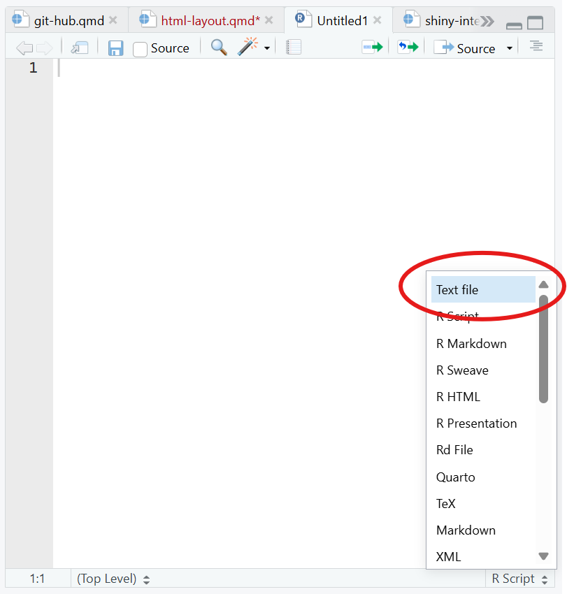
Prepare the bigliography

@Manual{rsoft,
    title = {R: A Language and Environment for Statistical Computing},
    author = {{R Core Team}},
    organization = {R Foundation for Statistical Computing},
    address = {Vienna, Austria},
    year = {2025},
    url = {https://www.R-project.org/}
}
@Book{ggplot,
    author = {Hadley Wickham},
    title = {ggplot2: Elegant Graphics for Data Analysis},
    publisher = {Springer-Verlag New York},
    year = {2016},
    isbn = {978-3-319-24277-4},
    url = {https://ggplot2.tidyverse.org}
}
@article{epifania2024,
  title={A guided tutorial on linear mixed-effects models for the analysis of accuracies and response times in experiments with fully crossed design.},
  author={Epifania, Ottavia M and Anselmi, Pasquale and Robusto, Egidio},
  journal={Psychological Methods},
  year={2024},
  publisher={American Psychological Association}, 
  doi={https://doi.org/10.1037/met0000708}
}

Mendeley, Zotero and similar software have built-in function for exporting the bib file. Read the related documentation of these softwares. Also Google Scholar provides the bibtex for each publication:

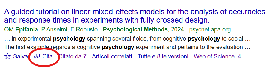
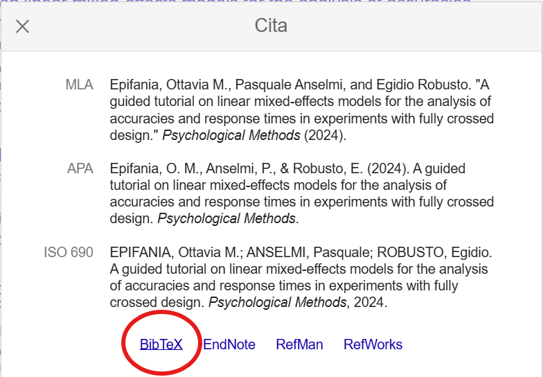
Then, from google scholar, you can copy & paste the citation on your bib file.

To call a reference:

@citaton-key

2.7 Citation keys

Key	Output
`@ggplot` does this	Wickman (2016) does this
`ggplot2 is an interesting package [@ggplot2]`	ggplot2 is an interesting package (Wickman, 2016)
`bla bla bla [@epifania2024; @ggplot2]`	bla bla bla (Epifania et al., 2024; Wickman, 2016)

Further details on the citation throughout a document are provided in Section 3.4.

3 Document layout

3.1 Columns

:::: {.columns}

::: {.column width="40%"}
I want some text in the left column
:::

::: {.column width="60%"}
And a picture in the right one 


:::

::::

I want some text in the left column

And a picture in the right one

The columns are most convenient in presentation files, while the grid (see Section 3.2) is the best option for changing the layout of a text document.

3.2 Grid

The document body is organized in 12 columns of equal width. This allows for a convenient and flexible environment for aligning the content.

The margins (left and right) are not counted within the 12-column space:

::: {.grid}

::: {.g-col-3}
Everything is fine
:::
  
::: {.g-col-2}
until
::: 
  
::: {.g-col-5}
the sum of the grid length is equal (or inferior) to 12
::: 
:::

Everything is fine

until

the sum of the grid length is equal (or inferior) to 12

3.3 Panel Tabset

::: {.panel-tabset}

## Aim

Here I present the aim of the study 

## Methods

Here I present the methods used to pursue the aim

## Results

And here I present the results

:::

Here I present the aim of the study

Here I present the methods used to pursue the aim

And here I present the results

3.4 Margins

Allows for placing images, code, references or equations in the margin of a document

For instance, I'm writing a document about peacocks, and I want a picture of a peacock and a little bit of text in the margin of the document, aligned with this text.

::: {.column-margin}
I want this picture displayed in the margin 


![](img/peacock.png)

:::

For instance, I’m writing a document about peacocks, and I want a picture of a peacock and a little bit of text in the margin of the document, aligned with this text.

I want this picture displayed in the margin

Even references can be placed in the margin, such that they appear alongside the text where they are cited.

Starting with the right settings in the YAML:

bibliography: biblio.bib
reference-location: margin
citation-location: margin

These lines of code force the citations to appear in the right margin. The citation key can happen as usual.

I want to cite the `ggplot2` package because it is the best package ever [@ggplot2]

I want to cite the ggplot2 package because it is the best package ever (Wickham 2016)

Wickham, Hadley. 2016. Ggplot2: Elegant Graphics for Data Analysis. Springer-Verlag New York. https://ggplot2.tidyverse.org.

Also equations can be put in the margins, so that they appear along with the text.

In this equation, we show how to stanrdarzie a raw $x$ value.

:::{.column-margin}

$$z = \dfrac{x - \mu}{\sigma}$$

:::

In this equation, we show how to stanrdarzie a raw \(x\) value.

\[z = \dfrac{x - \mu}{\sigma}\]

3.5 Callout blocks

:::{.callout-tip}
## Title of the tip

These are my two cents for you
:::

:::{.callout-note collapse=true}
## Two cents

These are my two cents for you
:::
  
:::{.callout-warning icon=false}
## Pay attention

Please mind the gap
:::

:::{.callout-caution}
## Danger!

This is dangerous!
:::

Title of the tip

These are my two cents for you

Two cents

These are my two cents for you

Pay attention

Please mind the gap

Danger!

This is dangerous!

4 Cross referencing

Everything in quarto can be cross-referenced with the correct key.

At this page https://quarto.org/docs/authoring/cross-references.html you can find all the details and help for a correct use of cross-referencing.

Label definition in the object to be referenced

{#obj-label}

Label referencing in text

@obj-label

Remember that the cross reference label depends on the language that has been set in the YAML (Section 1.8).

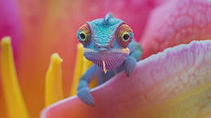
In @fig-cama there's a nice chameleon.

![This is an image](img/picture.jpg){#fig-cama}

In Figure 2 there’s a nice chameleon.

In @eq-reg we have an equation.

$$y = \beta_0 + \beta_1X_1 + \varepsilon$${#eq-reg}

In Equation 1 we have an equation.

\[y = \beta_0 + \beta_1X_1 + \varepsilon \tag{1}\]

## lang {#sec-lang}

bla bla bla

@sec-lang present the language definition throughout a document. Sections, subsections etc. are all cross-referenced with the prefix `sec`

Section 1.8 present the language definition throughout a document. Sections, subsections etc. are all cross-referenced with the prefix sec

It is also possible to cross reference R code, tables, and graphical output obtained from R code. These options are presented in the Code Chunk section.

5 `index.qmd`

As seen in the lesson on GitHub, the index.qmd (and specifically its rendered HTML) is used as the landing page of a document.

It can be configured as you wish, all the settings that have been presented in this lesson can be applied to index.qmd file.

Other pages can be linked to the landing page in the form of… links.

For instance, consider that you have an R project organized as follows:

my-project/
│
├── index.qmd
├── index.html
├── data/
│   └── mydata.csv
├── img/
│   ├── logo.png
│   ├── plot.jpg
│   └── illustration.svg
├── bibliography/
│   └── references.bib
└── docs/
    ├── about-me.qmd
    ├── about-me.html
    ├── cv.qmd
    └── cv.pdf

As the higher level, there is the index.qmd file and its rendered version in HTML (that is the one actually used as the landing page).

If you need to add other documents, you just need to link them in the landing page as a link, but indicating the path of the document.

Linkable page in the index

My cv is available at [this link](docs/cv.pdf), while [here](docs/about-me.html) you can find a brief summary of my research activity.

1 YAML

1.1 editor

1.2 editor: source

1.3 editor: visual

1.4 toc

1.5 Themes

1.6 Day

1.7 Night

1.8 lang

1.9 General Layout

2 Markdown formatting

2.1 Headings

2.2 Text Formatting

2.2.1 Formatting

2.2.2 Super/sub script

2.2.3 In line code

2.3 Links and images

2.4 Lists

2.5 Math

2.6 References

2.7 Citation keys

3 Document layout

3.1 Columns

3.2 Grid

3.3 Panel Tabset

3.4 Margins

3.5 Callout blocks

4 Cross referencing

5 index.qmd

1.1 `editor`

1.2 `editor: source`

1.3 `editor: visual`

1.4 `toc`

1.8 `lang`

5 `index.qmd`