Recap

Creating/naming objects

Creating/naming objects

Objects are created with the assignment arrow <-; = is only used to set the arguments of a function

x1 <- 3 # name <- object
x1

[1] 3

my_vector <- c(1, 2, 3)            # <- creates an object
mean(x = my_vector, na.rm = TRUE)  # = sets the arguments

[1] 2

Object names must start with a letter!! NOT “name” <- … but name <- …

Logical Operators

In R we can combine several relations to evaluate a given statement.

x <- 30 # Assign the value 30 to x.

Function	Name	Example	Result
&	Conjunction (AND)	x>25 & x<60	TRUE
|	Inclusive disjunction (OR)	x>25 | x>60	TRUE
!	Negation (NOT)	!(x<18)	TRUE

Vectors

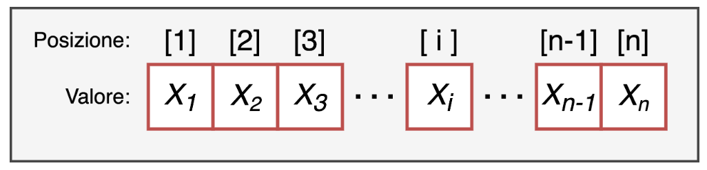
Vectors

• a value: the value of the element, which can be of any type, for example a number or a string of characters

• a position index: a positive integer that identifies its position within the vector.

Creating a vector

Vectors can be created with the c() command, writing inside the brackets the values of the elements in the desired order, separated by commas.

num_vect <- c(1,2,3,4)
# you can also use the seq() function
num_vect_seq <- seq(from = 1,to = 4, by = 1)

num_vect;num_vect_seq

[1] 1 2 3 4

[1] 1 2 3 4

char_vect <- c("R","R","R","ok")
# you can also use the rep() function
char_vect_rep <- c(rep("R", 3), "ok")

char_vect;char_vect_rep

[1] "R"  "R"  "R"  "ok"

[1] "R"  "R"  "R"  "ok"

Vector type

A vector must be made of elements all of the same type!

wrong <- c(1,2,3,"don't know", 4)
class(wrong)

[1] "character"

wrong

[1] "1"          "2"          "3"          "don't know" "4"         

Otherwise you “risk” everything being converted to character.

correct <- c(1,2,3,NA, 4)
class(correct)

[1] "numeric"

correct

[1]  1  2  3 NA  4

is.* & as.*

We can test or convert (when possible) the type of a vector with the is. & as. functions

is.character(char_vect)

[1] TRUE

as.numeric(char_vect) #!!

[1] NA NA NA NA

is.numeric(num_vect)

[1] TRUE

as.character(num_vect) #!!

[1] "1" "2" "3" "4"

logi_vect <- c(TRUE,FALSE,TRUE)
is.logical(logi_vect)

[1] TRUE

as.numeric(logi_vect)

[1] 1 0 1

Indexing

We can select, remove and extract elements simply by using the position index inside square brackets vector[pos]

# Create a vector of 20 random numbers drawn between 1 and 100
my_vect <- round(runif(n = 20,min = 1,max = 100))
my_vect

 [1]  8 57  8 54 50 42 85 48 22 34 45 48 34 43 39 15 30 61 85  6

my_vect[1] # extract the first element

[1] 8

my_vect[1:5] # extract the first 5 elements

[1]  8 57  8 54 50

my_vect[c(1,4,2,9)] # extract elements of our choice

[1]  8 54 57 22

my_vect[length(my_vect)] # last element (why?)

[1] 6

Negative indexing

In the same way, we can extract all the elements of the vector except some

my_vect[-c(1)] # all except the first element

 [1] 57  8 54 50 42 85 48 22 34 45 48 34 43 39 15 30 61 85  6

my_vect[-c(1:10)] # all except the first 10

 [1] 45 48 34 43 39 15 30 61 85  6

Logical Indexing

Indexing by position is the simplest and most intuitive approach. We can also select using TRUE and FALSE values: we can extract elements from the vector based on specific logical conditions

numbers <- 1:7
numbers

[1] 1 2 3 4 5 6 7

numbers[numbers<2]

[1] 1

Factors

Factors

Factors can be created either by converting a character vector with the as.factor() command or by explicitly creating a factor with the factor() command

char_vect <- rep(c("hello","ciao", "hola"), each = 2)
my_fact <- as.factor(char_vect)

my_fact2 <- factor(rep(c("hello","ciao", "hola"), each = 2))

my_fact == my_fact2

[1] TRUE TRUE TRUE TRUE TRUE TRUE

Properties of factors

In practice, they assign a label to an integer value:

typeof(my_fact)

[1] "integer"

as.integer(my_fact)

[1] 2 2 1 1 3 3

my_fact

[1] hello hello ciao  ciao  hola  hola 
Levels: ciao hello hola

Factor levels

Factors store levels() as metadata, regardless of which ones are actually present in the vector

levels(my_fact)

[1] "ciao"  "hello" "hola" 

my_fact2 <- my_fact[my_fact!="ciao"]
my_fact2

[1] hello hello hola  hola 
Levels: ciao hello hola

However, we can drop the levels that are no longer needed with the droplevels() command

droplevels(my_fact2)

[1] hello hello hola  hola 
Levels: hello hola

We can also rename the levels of a factor

# the factor I created
my_fact

[1] hello hello ciao  ciao  hola  hola 
Levels: ciao hello hola

# create another factor "my_fact_lev" identical to "my_fact"
my_fact_lev <- my_fact
my_fact_lev == my_fact

[1] TRUE TRUE TRUE TRUE TRUE TRUE

# rename the levels of the factor
levels(my_fact_lev) <- c("italian","english","spanish")

my_fact_lev

[1] english english italian italian spanish spanish
Levels: italian english spanish

my_fact

[1] hello hello ciao  ciao  hola  hola 
Levels: ciao hello hola

We can both reorder and rename the levels of a factor with the factor() function

my_fact

[1] hello hello ciao  ciao  hola  hola 
Levels: ciao hello hola

# by default levels are assigned in alphabetical order
as.integer(my_fact)

[1] 2 2 1 1 3 3

new_fact <- factor(my_fact, levels = c("hello","ciao","hola"))
new_fact

[1] hello hello ciao  ciao  hola  hola 
Levels: hello ciao hola

as.integer(new_fact)

[1] 1 1 2 2 3 3

new_fact2 <- factor(my_fact, levels = c("hello","ciao","hola"),
                   labels = c("english","italian","spanish"))
new_fact2

[1] english english italian italian spanish spanish
Levels: english italian spanish

Remember: the levels argument inside the factor() function is used to reorder the levels of the factor, while the levels() function renames them, it does not reorder them!

# the factor I created
my_fact

[1] hello hello ciao  ciao  hola  hola 
Levels: ciao hello hola

as.integer(my_fact)

[1] 2 2 1 1 3 3

levels(my_fact) <- c("hello","ciao","hola")

# What do you notice compared to the my_fact vector shown above?
my_fact

[1] ciao  ciao  hello hello hola  hola 
Levels: hello ciao hola

as.integer(my_fact)

[1] 2 2 1 1 3 3

Lists

Lists

Lists are flexible structures that can contain objects of different types and different sizes (each element can itself be a list)

my_list <- list("hello!", 1:3, c(TRUE,FALSE),
               list("hello!", 1:3, c(TRUE,FALSE)))
str(my_list)

List of 4
 $ : chr "hello!"
 $ : int [1:3] 1 2 3
 $ : logi [1:2] TRUE FALSE
 $ :List of 3
  ..$ : chr "hello!"
  ..$ : int [1:3] 1 2 3
  ..$ : logi [1:2] TRUE FALSE

Lists

Although a list is one-dimensional, it develops in depth

str(my_list)

List of 4
 $ : chr "hello!"
 $ : int [1:3] 1 2 3
 $ : logi [1:2] TRUE FALSE
 $ :List of 3
  ..$ : chr "hello!"
  ..$ : int [1:3] 1 2 3
  ..$ : logi [1:2] TRUE FALSE

Lists

First Level: list

str(my_list[2])

List of 1
 $ : int [1:3] 1 2 3

Second Level: numeric vector

str(my_list[[2]])

 int [1:3] 1 2 3

Third Level: integer

str(my_list[[2]][1]) # integer

 int 1

Lists

We can assign names to the elements of a list…

my_list_nam <- list(word = "hello!",numbers =  1:3,
                   logical = c(TRUE,FALSE),
               list = list("hello!", 1:3, c(TRUE,FALSE)))
my_list_nam

$word
[1] "hello!"

$numbers
[1] 1 2 3

$logical
[1]  TRUE FALSE

$list
$list[[1]]
[1] "hello!"

$list[[2]]
[1] 1 2 3

$list[[3]]
[1]  TRUE FALSE

Lists

… and access them by calling them by “name” with the $ operator

my_list_nam$word

[1] "hello!"

my_list_nam$list # list created as an element of the list

[[1]]
[1] "hello!"

[[2]]
[1] 1 2 3

[[3]]
[1]  TRUE FALSE

Lists - Attributes

Like vectors, lists also have a length (length()) and possibly names (names()). The str() (structure) command is very useful for lists because it gives an overview of their structure:

length(my_list_nam); names(my_list_nam)

[1] 4

[1] "word"    "numbers" "logical" "list"   

str(my_list_nam)

List of 4
 $ word   : chr "hello!"
 $ numbers: int [1:3] 1 2 3
 $ logical: logi [1:2] TRUE FALSE
 $ list   :List of 3
  ..$ : chr "hello!"
  ..$ : int [1:3] 1 2 3
  ..$ : logi [1:2] TRUE FALSE

Lists - Indexing

The difference between the square brackets is whether we want to subset the list, getting another list, or directly access the inner element:

my_list_nam[1] # getting another list

$word
[1] "hello!"

my_list_nam[[1]] # accessing the inner element

[1] "hello!"

Lists - Indexing

If we want to select several elements (i.e. actually subset the list) we must always use single square brackets:

# list made of the first two elements of my_list_nam
my_list_nam[1:2]

$word
[1] "hello!"

$numbers
[1] 1 2 3

Lists - Nested Indexing

Lists have a one-dimensional structure that can develop in depth. To select nested elements we can chain several brackets:

my_list_nam[[4]]

[[1]]
[1] "hello!"

[[2]]
[1] 1 2 3

[[3]]
[1]  TRUE FALSE

my_list_nam[[4]][[1]]

[1] "hello!"

my_list_nam[[4]][[2]]

[1] 1 2 3

Matrices

Matrices

Matrices are a two-dimensional data structure (characterized by 2 dimensions, dim()), where the number of rows is dimension 1 and the number of columns is dimension 2.

my_mat <- matrix(data = 1:10, nrow = 2, ncol = 5, byrow = FALSE)
my_mat

     [,1] [,2] [,3] [,4] [,5]
[1,]    1    3    5    7    9
[2,]    2    4    6    8   10

matrix(data = 1:10, nrow = 2, ncol = 5, byrow = TRUE)

     [,1] [,2] [,3] [,4] [,5]
[1,]    1    2    3    4    5
[2,]    6    7    8    9   10

Matrices - Properties

• They can contain only one type of data

• Since they are two-dimensional, we need two position indices (rows and columns) to identify an element

• They can be seen as a set of single vectors

Matrices - Properties

The number of rows and columns does not have to be the same (square matrix), but the size of the matrix must be compatible with the data vector:

matrix(data = 1:10, ncol = 3, nrow = 3)

Warning in matrix(data = 1:10, ncol = 3, nrow = 3): data length [10] is not a
sub-multiple or multiple of the number of rows [3]

     [,1] [,2] [,3]
[1,]    1    4    7
[2,]    2    5    8
[3,]    3    6    9

Matrices

What does R do by default?

matrix(data = 1:10, ncol = 3, nrow = 3)

     [,1] [,2] [,3]
[1,]    1    4    7
[2,]    2    5    8
[3,]    3    6    9

matrix(data = 1:2, ncol = 3, nrow = 3)

     [,1] [,2] [,3]
[1,]    1    2    1
[2,]    2    1    2
[3,]    1    2    1

warnings: the function informs us about something potentially problematic, but (more or less!!) everything is fine

Matrices - Indexing

To identify one or more elements of a matrix we need row and/or column indices separated by a comma, again inside square brackets: matrix[row, column]

my_mat

     [,1] [,2] [,3] [,4] [,5]
[1,]    1    3    5    7    9
[2,]    2    4    6    8   10

my_mat[1,1]

[1] 1

Matrices - Indexing

We can also select an entire row or column

my_mat[1,]

[1] 1 3 5 7 9

my_mat[,1]

[1] 1 2

Matrices - Indexing

As with vectors, here too we can apply logical indexing:

my_mat>2

      [,1] [,2] [,3] [,4] [,5]
[1,] FALSE TRUE TRUE TRUE TRUE
[2,] FALSE TRUE TRUE TRUE TRUE

# All the elements greater than two
my_mat[my_mat>2]

[1]  3  4  5  6  7  8  9 10

Vectors and Matrices

Vectors are created with the c() function and can be concatenated using the same function:

my_vect1 <- c(1:4); my_vect2 <- c(5:10)
my_vect12 <- c(my_vect1,my_vect2)
my_vect12

 [1]  1  2  3  4  5  6  7  8  9 10

Matrices

Similarly, matrices can be joined together with the cbind() and rbind() commands:

my_mat <- matrix(1:4,2,2)

cbind(my_mat, my_mat)

     [,1] [,2] [,3] [,4]
[1,]    1    3    1    3
[2,]    2    4    2    4

rbind(my_mat, my_mat)

     [,1] [,2]
[1,]    1    3
[2,]    2    4
[3,]    1    3
[4,]    2    4

Dataframe

Dataframe

The dataframe is the most “complex”, useful and powerful structure in R. Intuitively it is an excel sheet, while from R’s point of view it is a type of list with some properties/restrictions

• each element of the list is a vector with an associated name (aka a column)
• each list/column must have the same number of elements
• as a consequence, each row has the same number of elements (rectangular structure)

Creating a dataframe

With the data.frame() function we can create a dataframe…

# Create a dataframe with 3 columns
my_df <- data.frame( col1 = 1:4, col2 = letters[1:4],
                    col3 = rnorm(4))
my_df

  col1 col2       col3
1    1    a  1.0448101
2    2    b  0.1357442
3    3    c  0.1539800
4    4    d -1.1813148

Attributes

The dataframe has both the attributes of a list, i.e. the names, and the attributes of a matrix, i.e. the dimensions (rows and columns)

typeof(my_df)

[1] "list"

attributes(my_df)

$names
[1] "col1" "col2" "col3"

$class
[1] "data.frame"

$row.names
[1] 1 2 3 4

dim(my_df)

[1] 4 3

Indexing

We can use either square brackets [] or the dollar sign $

my_df[1] # extract a 4x1 data.frame

  col1
1    1
2    2
3    3
4    4

my_df[[1]]# extract the first column of the data.frame

[1] 1 2 3 4

my_df$col1# extract the first column of the data.frame

[1] 1 2 3 4

my_df[1,1]# extract the first element of the first column of the data.frame

[1] 1

Indexing - Relational operators

One of the most common operations you will deal with is extracting/evaluating a subset of the values in your dataset:

# keep only the rows where the values of column1 are greater than 2
my_df[my_df$col1 > 2, ]

  col1 col2      col3
3    3    c  0.153980
4    4    d -1.181315

my_df[my_df[1] > 2, ]

  col1 col2      col3
3    3    c  0.153980
4    4    d -1.181315

Examples

  col1 col2       col3
1    1    a  1.0448101
2    2    b  0.1357442
3    3    c  0.1539800
4    4    d -1.1813148

• my_df[my_df$col1 > 1 & my_df$col1 < 4, ]
  • 2 b -0.5630882
  • 3 c -0.5672335
• my_df[my_df$col1== 1, "col3"]
  • -1.481937
• my_df[my_df$col1== 1, 3]
  • -1.481937

Indexing

There are also alternative, more compact ways of indexing. For example, using the subset() function:

subset(iris, subset = Species == "setosa" & Petal.Length > 1.7)

   Sepal.Length Sepal.Width Petal.Length Petal.Width Species
25          4.8         3.4          1.9         0.2  setosa
45          5.1         3.8          1.9         0.4  setosa

equivalent to:

iris[iris$Species == "setosa" & iris$Petal.Length > 1.7,]

   Sepal.Length Sepal.Width Petal.Length Petal.Width Species
25          4.8         3.4          1.9         0.2  setosa
45          5.1         3.8          1.9         0.4  setosa

We can also select columns rather than rows with the select argument:

head(subset(iris, select = c(Sepal.Length, Species)), n = 3)

  Sepal.Length Species
1          5.1  setosa
2          4.9  setosa
3          4.7  setosa

We can also combine the two:

head(subset(iris, Species == "setosa" & Sepal.Length > 4,
             c(Sepal.Length, Species)), n = 3)

  Sepal.Length Species
1          5.1  setosa
2          4.9  setosa
3          4.7  setosa

equivalent to:

head(iris[iris$Species == "setosa" & iris$Sepal.Length > 4,
          c("Sepal.Length","Species")],n = 3)

  Sepal.Length Species
1          5.1  setosa
2          4.9  setosa
3          4.7  setosa

$$$$$$

Most of the time you will access variables with the $ operator. This command can also be used to create a new variable…

iris$sum <- iris$Sepal.Length + iris$Sepal.Width
str(iris)

'data.frame':   150 obs. of  6 variables:
 $ Sepal.Length: num  5.1 4.9 4.7 4.6 5 5.4 4.6 5 4.4 4.9 ...
 $ Sepal.Width : num  3.5 3 3.2 3.1 3.6 3.9 3.4 3.4 2.9 3.1 ...
 $ Petal.Length: num  1.4 1.4 1.3 1.5 1.4 1.7 1.4 1.5 1.4 1.5 ...
 $ Petal.Width : num  0.2 0.2 0.2 0.2 0.2 0.4 0.3 0.2 0.2 0.1 ...
 $ Species     : Factor w/ 3 levels "setosa","versicolor",..: 1 1 1 1 1 1 1 1 1 1 ...
 $ sum         : num  8.6 7.9 7.9 7.7 8.6 9.3 8 8.4 7.3 8 ...

EXAM

https://etherpad.wikimedia.org/p/arca-corsoR