Recap - Day 1

Objects, operators and vectors

Working directory

Working directory

The folder where R reads and saves files, unless we tell it otherwise

getwd()                              # where am I working?
# change the working directory
setwd("/Users/tita/Desktop/introR")
  • relative path: starts from the working directory
# the file is inside the working directory
data <- read.csv("prova.csv")
  • absolute path: the full address of the file on the computer
data <- read.csv("/Users/tita/Desktop/prova.csv")

R Projects

The best solution: an R Project (File > New Project...)

  • it sets the working directory automatically to the project folder
  • so we can always use relative paths: the code works on any computer
  • it keeps all the files of a project (scripts, data, results) together

Open the project by double-clicking the .Rproj file: RStudio starts in the right folder

Objects

Creating an object

We create an object with the assignment arrow <-: name <- value

age <- 25
age            # to see its value, write its name
[1] 25

We can overwrite it, or use it to create new objects:

age <- age + 1
age_in_months <- age * 12
age_in_months
[1] 312

Naming objects

  • names must start with a letter: x1 yes, 1x no
  • R is case-sensitive: Name and name are two different objects
Name <- "Margherita"
name <- "margherita"
Name == name
[1] FALSE

The objects we create live in the environment: ls() lists them, rm() removes one, rm(list =ls()) removes all

rm(name)
ls()
[1] "age"           "age_in_months" "Name"         
rm(list = ls())
ls()
character(0)

Data types

class(3.14)        # numeric (double)
[1] "numeric"
class(5L)          # integer
[1] "integer"
class("hello")     # character: always in quotes
[1] "character"
class(TRUE)        # logical: TRUE or FALSE
[1] "logical"

Careful with quotes: "5" is text, not a number!

"5" + 1
Error in `"5" + 1`:
! non-numeric argument to binary operator

Operators

Mathematical operators

operator what it does example result
+ - addition, subtraction 5 + 2 - 1 6
* / multiplication, division 6 * 2 / 4 3
^ power 2 ^ 3 8
%% remainder of the division 9 %% 2 1

R follows the order of operations of mathematics: use parentheses when in doubt

1 + 2 * 3
[1] 7
(1 + 2) * 3
[1] 9

Mathematical functions

sqrt(16)            # square root
[1] 4
abs(-7)             # absolute value
[1] 7
round(3.14159, 2)   # round to 2 decimals
[1] 3.14
exp(1)              # exponential
[1] 2.718282
log(10)             # natural logarithm
[1] 2.302585

Relational operators

They compare two values and return TRUE or FALSE

operator meaning example result
== != equal, different 5 == 5 TRUE
> >= greater (or equal) 5 > 7 FALSE
< <= less (or equal) 5 <= 5 TRUE
%in% is it contained in…? 2 %in% c(1, 2, 3) TRUE

Remember: = (or <-) assigns, == compares!

Logical operators

They combine several conditions

x <- 30
x > 25 & x < 60    # AND: both must be TRUE
[1] TRUE
x < 18 | x > 60    # OR: at least one must be TRUE
[1] FALSE
!(x > 25)          # NOT: inverts TRUE and FALSE
[1] FALSE

Order of evaluation: mathematical, then relational, then logical operators

2 * 3 > 5 & 10 %% 2 == 0
[1] TRUE

TRUE and FALSE are numbers

In calculations, TRUE counts as 1 and FALSE as 0

TRUE + TRUE
[1] 2
answers <- c(TRUE, FALSE, TRUE, TRUE)
sum(answers)    # how many TRUE?
[1] 3
mean(answers)   # proportion of TRUE
[1] 0.75

Very useful to count how many values meet a condition:

scores <- c(18, 25, 30, 22, 27)
sum(scores >= 25)   # how many scores are at least 25?
[1] 3

Vectors

What is a vector

A one-dimensional sequence of elements, all of the same type. Each element has a value and a position.
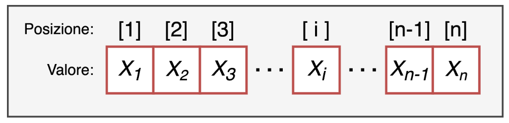
temps <- c(12, 18, 25, 31, 7)
length(temps)     # number of elements
[1] 5

Creating vectors

c(4, 8, 15)                         # combine values
[1]  4  8 15
1:5                                 # integers from 1 to 5
[1] 1 2 3 4 5
seq(from = 0, to = 10, by = 2)       # sequence with a step
[1]  0  2  4  6  8 10
seq(from = 0, to = 1, length.out = 5) # sequence with a length
[1] 0.00 0.25 0.50 0.75 1.00
rep(c("x", "y"), times = 2)          # repeat the whole vector
[1] "x" "y" "x" "y"
rep(c("x", "y"), each = 2)           # repeat each element
[1] "x" "x" "y" "y"

One type only

If we mix types, R converts everything to one type (usually character):

mixed <- c(1, 2, "three")
mixed
[1] "1"     "2"     "three"
class(mixed)
[1] "character"

A missing value is written NA (not “NA”!) and does not change the type:

with_na <- c(1, 2, NA, 4)
class(with_na)
[1] "numeric"

Testing and converting: is. and as.

is. tests the type, as. converts it (when possible)

nums <- c(1, 0, 3)
is.numeric(nums)
[1] TRUE
is.character(nums)
[1] FALSE
as.character(nums)
[1] "1" "0" "3"
as.logical(nums)       # 0 is FALSE, others TRUE
[1]  TRUE FALSE  TRUE
# what cannot be converted becomes NA
as.numeric(c("1", "2", "three"))
Warning: NAs introduced by coercion
[1]  1  2 NA

Operations on vectors

Operations are applied element by element:

temps <- c(12, 18, 25, 31, 7)
temps * 9/5 + 32        # Celsius to Fahrenheit
[1] 53.6 64.4 77.0 87.8 44.6
temps > 20              # one TRUE/FALSE for each element
[1] FALSE FALSE  TRUE  TRUE FALSE

Summary functions return one value for the whole vector:

mean(temps); sd(temps); max(temps); sum(temps)
[1] 18.6
[1] 9.659193
[1] 31
[1] 93

Missing values: NA

scores <- c(18, NA, 30, 22, NA)
mean(scores)                 # one NA makes the result NA
[1] NA
mean(scores, na.rm = TRUE)   # remove the NAs before computing
[1] 23.33333
is.na(scores)          # which elements are NA?
[1] FALSE  TRUE FALSE FALSE  TRUE
sum(is.na(scores))     # how many?
[1] 2

Indexing

Indexing by position

Square brackets vector[position] select elements:

temps <- c(12, 18, 25, 31, 7)
temps[2]                  # the second element
[1] 18
temps[c(1, 3)]            # the first and the third
[1] 12 25
temps[2:4]                # from the second to the fourth
[1] 18 25 31
temps[length(temps)]      # the last one
[1] 7

Negative indexing

A negative position excludes that element:

temps
[1] 12 18 25 31  7
temps[-1]                 # all except the first
[1] 18 25 31  7
temps[-c(1, 2)]           # all except the first two
[1] 25 31  7
temps[-length(temps)]     # all except the last
[1] 12 18 25 31

Indexing by name

If the elements have names, we can select them by name:

names(temps) <- c("Mon", "Tue", "Wed", "Thu", "Fri")
temps
Mon Tue Wed Thu Fri 
 12  18  25  31   7 
temps["Wed"]
Wed 
 25 
temps[c("Mon", "Fri")]
Mon Fri 
 12   7 

Logical indexing

A logical condition inside the brackets keeps the elements where it is TRUE:

temps > 20                  # the condition, for each element
  Mon   Tue   Wed   Thu   Fri 
FALSE FALSE  TRUE  TRUE FALSE 
temps[temps > 20]           # only the elements where it is TRUE
Wed Thu 
 25  31 
temps[temps > 10 & temps < 30]
Mon Tue Wed 
 12  18  25 

which() gives the positions where the condition is TRUE:

which(temps > 20)
Wed Thu 
  3   4 

Indexing to modify

Selecting elements and assigning a new value modifies only those elements:

scores <- c(18, NA, 30, 22, NA)
scores[1] <- 20                   # change the first element
scores
[1] 20 NA 30 22 NA
scores[is.na(scores)] <- 0        # replace the NAs with 0
scores
[1] 20  0 30 22  0
scores[scores < 21] <- 21         # raise the low scores to 21
scores
[1] 21 21 30 22 21

Summary

to… use
know / change the wd getwd() / setwd(), or an R Project
create an object name <- value
compare / combine conditions == != > < %in% / & | !
create a vector c(), :, seq(), rep()
test / convert a type is.numeric(), as.character(), …
deal with missing values is.na(), na.rm = TRUE
select elements x[2], x[-2], x["name"], x[x > 5], which()
modify elements x[condition] <- new_value

Now let’s practice!


Open this link and keep it open:

https://etherpad.wikimedia.org/p/arca-corsoR