EXTRA

Preprocessing

Steps before data analysis

  • Load the dataset
  • Check the structure, missing data, odd data
  • Visualize

Loading packages

As a first step, it is good practice to load the required packages (and first install them if they are not installed yet).

packages <- c("readr", "tidyverse", "ggplot2", "ggpubr")
sapply(packages, require, character.only = T)
    readr tidyverse   ggplot2    ggpubr 
     TRUE      TRUE      TRUE      TRUE 

Loading the dataset

You may not have a single dataset with all the subjects together, but instead have to load one dataset per subject and combine them afterwards. For this kind of operation the map_dfr function is useful (similar to apply, it is in the purrr package, from the magic world of the tidyverse).

Loading the dataset

list.files lets you search and see which files match a specific pattern. In my case I go into the folder and load all the data in .csv format (I use the head function to show you the first 6)

[1] "dataRaw/GNG100_1_SD.csv" "dataRaw/GNG101_1_FS.csv"
[3] "dataRaw/GNG102_1_SD.csv" "dataRaw/GNG103_1_FS.csv"
[5] "dataRaw/GNG104_1_FS.csv" "dataRaw/GNG106_1_FS.csv"

Loading the dataset

I apply the map_dfr function to all the files just obtained with the list.files function…

d <- list.files(path = "dataRaw", pattern = "*.csv", 
               full.names = TRUE)%>%
  map_dfr(~read_csv(.x)) 
Error in `dplyr::bind_rows()`:
! Can't combine `..37$session` <double> and `..38$session` <character>.

Loading the dataset

Error in dplyr::bind_rows(): ! Can’t combine ..37$session and ..38$session .

For some reason, in some files the session information is read as double instead of character. So inside map_dfr I also add mutate

d <- list.files(path = "dataRaw", pattern = "*.csv", 
             full.names = TRUE) %>% 
  map_dfr(~read_csv(.x) %>% 
            mutate(condition = as.character(condition),
                   session = as.character(session)) %>%
            subset(RUN >= 1)) # remove all the extra rows I don't need

Looking at the variables

For example, I check that the subjects used the assigned IDs. The unique() function is very useful because it returns a vector without duplicated elements (in my dataset I had 448 trials per subject, so each id is repeated 448 times).

unique(d$participant)
 [1] "GN100"  "GNG101" "GNG102" "GNG103" "GNG104" "GNG106" "GNG107" "GNG15" 
 [9] "GNG16"  "GNG17"  "GNG18"  "GNG19"  "GNG20"  "GNG21"  "GNG22"  "GNG23" 
[17] "GNG24"  "GNG25"  "GNG26"  "GNG27"  "GNG28"  "GNG29"  "GNG33"  "GNG34" 
[25] "GNG35"  "GNG36"  "GNG37"  "GNG38"  "GNG39"  "GNG40"  "GNG41"  "GNG42" 
[33] "GNG43"  "GNG44"  "GNG45"  "GNG46"  "GNG47"  "GNG48"  "GNG49"  "GNG50" 
[41] "GNG53"  "GNG54"  "GNG55"  "GNG56"  "GNG58"  "GNG59"  "GNG60"  "GNG61" 
[49] "GNG62"  "GNG63"  "GNG64"  "GNG66"  "GNG67"  "GNG68"  "GNG69"  "GNG70" 
[57] "GNG71"  "GNG73"  "GNG74"  "GNG76"  "GNG78"  "GNG79"  "GNG80"  "GNG81" 
[65] "GNG82"  "GNG83"  "GNG87"  "GNG85"  "GNG86"  "GNG88"  "GNG89"  "GNG90" 
[73] "GNG92"  "GNG93"  "GNG94"  "GNG95"  "GNG96"  "GNG97"  "GNG98" 

The grep() function searches for a pattern inside a string; in this case the subject id was supposed to be GNG…

grep(pattern = "GNG", x = unique(as.factor(d$participant)))
 [1]  2  3  4  5  6  7  8  9 10 11 12 13 14 15 16 17 18 19 20 21 22 23 24 25 26
[26] 27 28 29 30 31 32 33 34 35 36 37 38 39 40 41 42 43 44 45 46 47 48 49 50 51
[51] 52 53 54 55 56 57 58 59 60 61 62 63 64 65 66 67 68 69 70 71 72 73 74 75 76
[76] 77 78 79
unique(d$participant)[-c(grep(pattern = "GNG", x = unique(d$participant)))]
[1] "GN100"
d$id <- factor(case_when(d$participant == "GN100"~ "GNG100",
                        .default = d$participant))

…and that they entered the experimental condition correctly…

unique(d$condition)
[1] "SD"            "FS"            "sd"            "fs"           
[5] "FF"            "CONDIZIONE SD" "CONDIZIONE FS"
d$C <- factor(case_when(d$condition == "CONDIZIONE FS" ~ "FS",
                       d$condition == "FF" ~ "FS",
                       d$condition == "fs" ~ "FS",
                       d$condition == "sd" ~ "SD",
                       d$condition == "FS" ~ "FS",
                       d$condition == "CONDIZIONE SD" ~ "SD",
                       d$condition == "SD" ~ "SD"))

Tidying the dataset

I convert the variables I am interested in to factors, and keep only those I need for visualization and analysis. We can use mutate() to mutate/change the variable type, and select() to select the variables of interest:

dat <- d %>% 
  mutate(P = factor(LW_P),
         target = factor(target_col),
         B = factor(B),
         rt = target_kb.rt,
         resp = target_kb.keys,
         Trial = TRIAL.thisN + 1)|>
  select(id, P, target, C, B, rt, resp, Trial)

Check

A quick check of the structure of the dataset

str(dat)
tibble [35,392 × 8] (S3: tbl_df/tbl/data.frame)
 $ id    : Factor w/ 79 levels "GNG100","GNG101",..: 1 1 1 1 1 1 1 1 1 1 ...
 $ P     : Factor w/ 3 levels "0.2","0.5","0.8": 1 1 1 1 1 1 1 1 1 1 ...
 $ target: Factor w/ 2 levels "go.png","nogo.png": 2 2 1 2 2 2 1 2 2 2 ...
 $ C     : Factor w/ 2 levels "FS","SD": 2 2 2 2 2 2 2 2 2 2 ...
 $ B     : Factor w/ 12 levels "1","2","3","4",..: 1 1 1 1 1 1 1 1 1 1 ...
 $ rt    : num [1:35392] NA NA 0.396 NA NA NA 0.377 NA NA NA ...
 $ resp  : chr [1:35392] NA NA "space" NA ...
 $ Trial : num [1:35392] 1 2 3 4 5 6 7 8 9 10 ...

Adding an accuracy variable

If there is a response and the trial was Go, then correct (1); if there is a response and the trial was NoGo, then wrong (0)…

dat$acc <- case_when(dat$target == "nogo.png" & dat$resp == "space" ~ 0,
                    dat$target == "nogo.png" &  is.na(dat$resp) ~ 1,
                    dat$target == "go.png" & dat$resp == "space" ~ 1,
                    dat$target == "go.png" & is.na(dat$resp) ~ 0,
                    TRUE ~ 3)

# check
sum(dat$acc == 3)
[1] 0

Excluding subjects

Sometimes some subjects are excluded a priori because they did not follow the “rules” of the experiment; in this case you can exclude them right away

dat_clean <- subset(dat, 
                        # PSQI = 14
                        id != "GNG82" & 
                        # not respect sleep schedule
                        id != "GNG16" & 
                        id != "GNG21" & id != "GNG40" & 
                        id != "GNG46" & id != "GNG51" &
                        id != "GNG52"& id != "GNG58" &
                        id != "GNG65" & id != "GNG72" &
                        id != "GNG75" &  id != "GNG83"&
                        id != "GNG92" & id != "GNG95"&
                        id != "GNG96" & id != "GNG105")

# you can also create a vector of IDs to exclude and then use %in%

Excluding subjects

In my case I also wanted to exclude everyone with accuracy below 70%. To compute descriptive statistics, the group_by and summarise functions from the dplyr package (tidyverse again) are very useful

summ_acc <- dat_clean %>% 
  group_by(id, target)%>%
  summarise(acc_mean = round(mean(acc),2),
            n = n())

# subjects GNG102 GNG38  GNG59  GNG59 had very low accuracy
summ_acc$id[which(summ_acc$acc_mean < .7)]
[1] GNG102 GNG102 GNG38  GNG59  GNG59 
79 Levels: GNG100 GNG101 GNG102 GNG103 GNG104 GNG106 GNG107 GNG15 ... GNG98

So I exclude them using the negation of %in% (which checks whether an element is present in a vector)

dat_clean2 <- subset(dat_clean, 
                  !(id %in% summ_acc$id[which(summ_acc$acc_mean < .7)]))

I check that the ids with accuracy below .7 are indeed gone

sum(dat_clean2$id %in% summ_acc$id[which(summ_acc$acc_mean < .7)])
[1] 0

After cleaning the data it is good to check how much information is left, for example the number of subjects per group. n_distinct counts the number of unique combinations..

dat_clean2 %>%
  group_by(C) %>%
  summarise(n_subj = n_distinct(id))
# A tibble: 2 × 2
  C     n_subj
  <fct>  <int>
1 FS        34
2 SD        32

Now let’s visualize them

One of the best packages for data visualization is ggplot2; you can do practically anything with it.

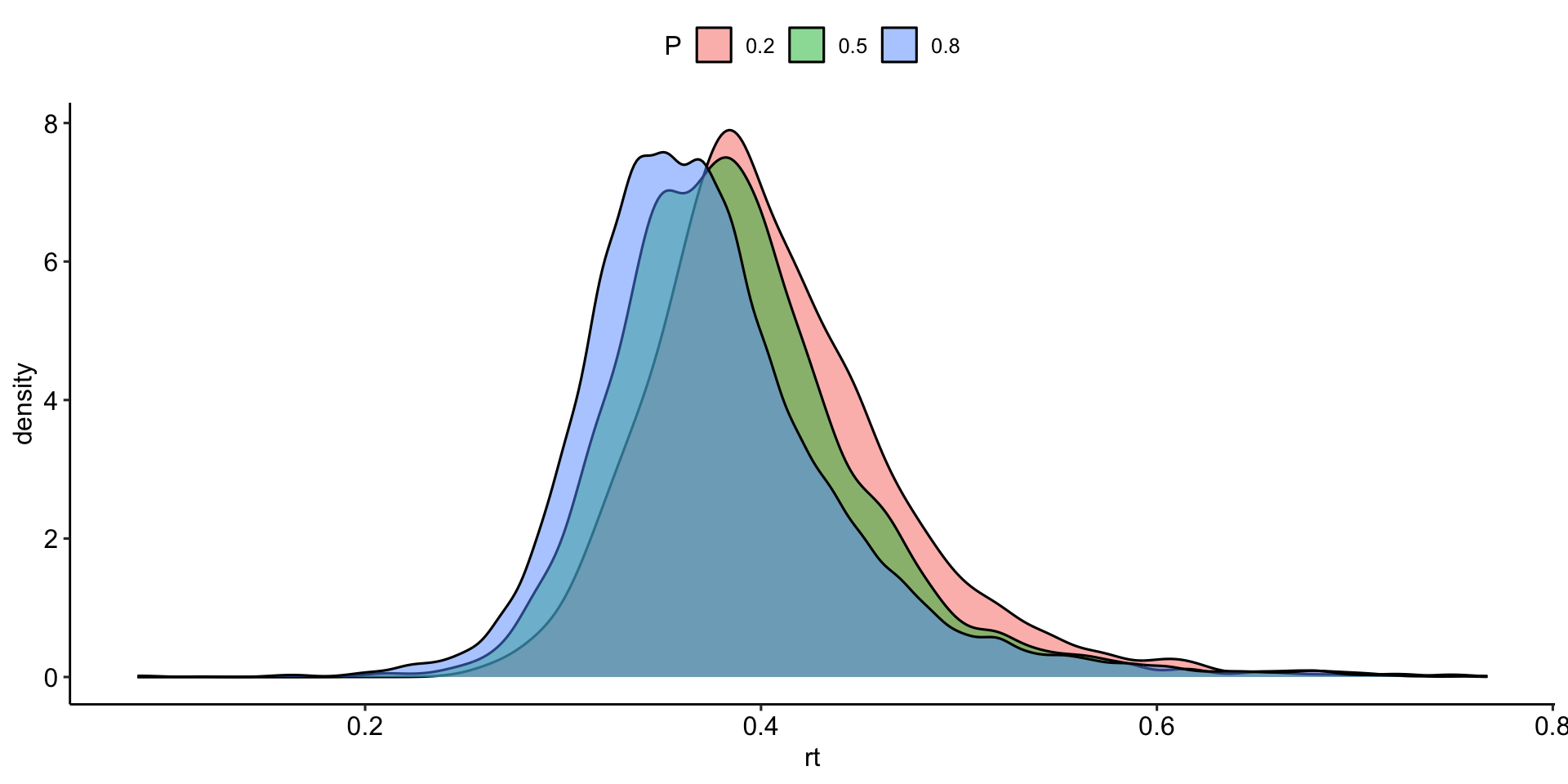
The first reason to visualize data is to see their distribution, the presence of extreme values… ggplot takes as input which variables to use for x and y (or only one of the two, depending on what we want to plot); I can also specify colors and various other things we will see…

theme_set(theme_pubr())

dat_clean2 %>% subset(target == "go.png") %>% 
  ggplot(aes(x= rt, fill = P))+
  geom_density(alpha = .5)

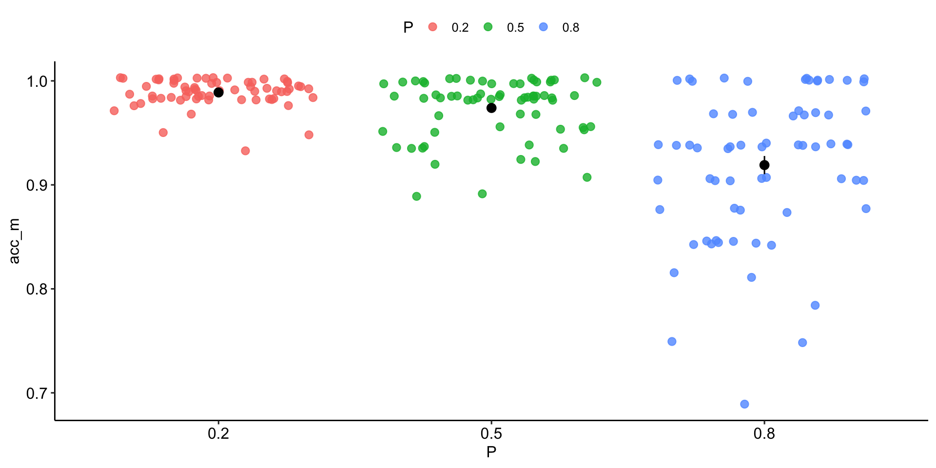
Accuracy

dat_clean2 %>% subset(target == "nogo.png") %>% 
  group_by(id,P)%>% # group the dataset by id and P
  # compute the mean accuracy per condition/subject
  summarise(acc_m = mean(acc))%>% # 
  ggplot(aes(y= acc_m, x = P, color = P))+
  geom_jitter(alpha = .8, size = 2.5)+ # dots
  stat_summary(color = "black") # add mean and se

Customization

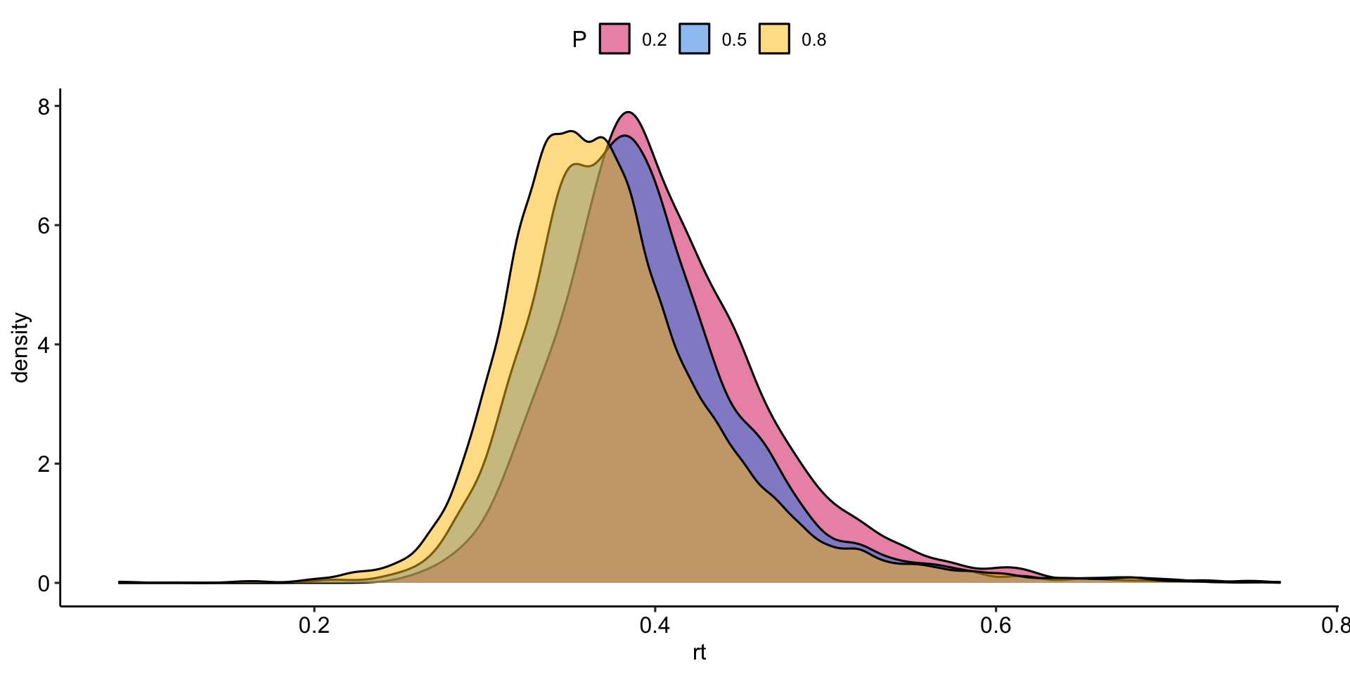
A simple and nice thing to do is to create your own color palette to use whenever you want in your plots. You can define it at the beginning or write it in a separate script and load it with the source() command, as we saw for functions. At this link you can find lots of (colorblind-friendly) colors

my_pal <- list(
  pal1 = c("#D81B60","#1E88E5", "#FFC107", "#004D40"),
  pal2 = c("#580646","#3CA756", "#CE597A"),
  pal = c("#D81B60", "#004D40", "#1E88E5", "#FFC107",
          "#580646","#3CA756", "#CE597A")
)
dat_clean2 %>% subset(target == "go.png") %>% 
  ggplot(aes(x= rt, fill = P))+
  geom_density(alpha = .5)+
  scale_fill_manual(values = my_pal$pal1) # use my palette 

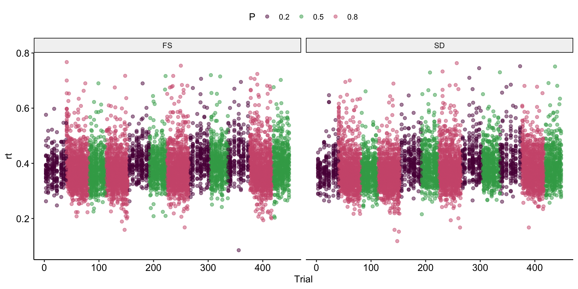
With the facet_wrap() function we can split the plot, for example with one panel for each group in my case, using ~ C

dat_clean2 %>% subset(target == "go.png") %>% 
  ggplot(aes(y= rt, x = Trial, color = P))+
  geom_point(alpha = .5)+facet_wrap(~ C) + # facet_wrap splits into panels
  scale_color_manual(values = my_pal$pal2)
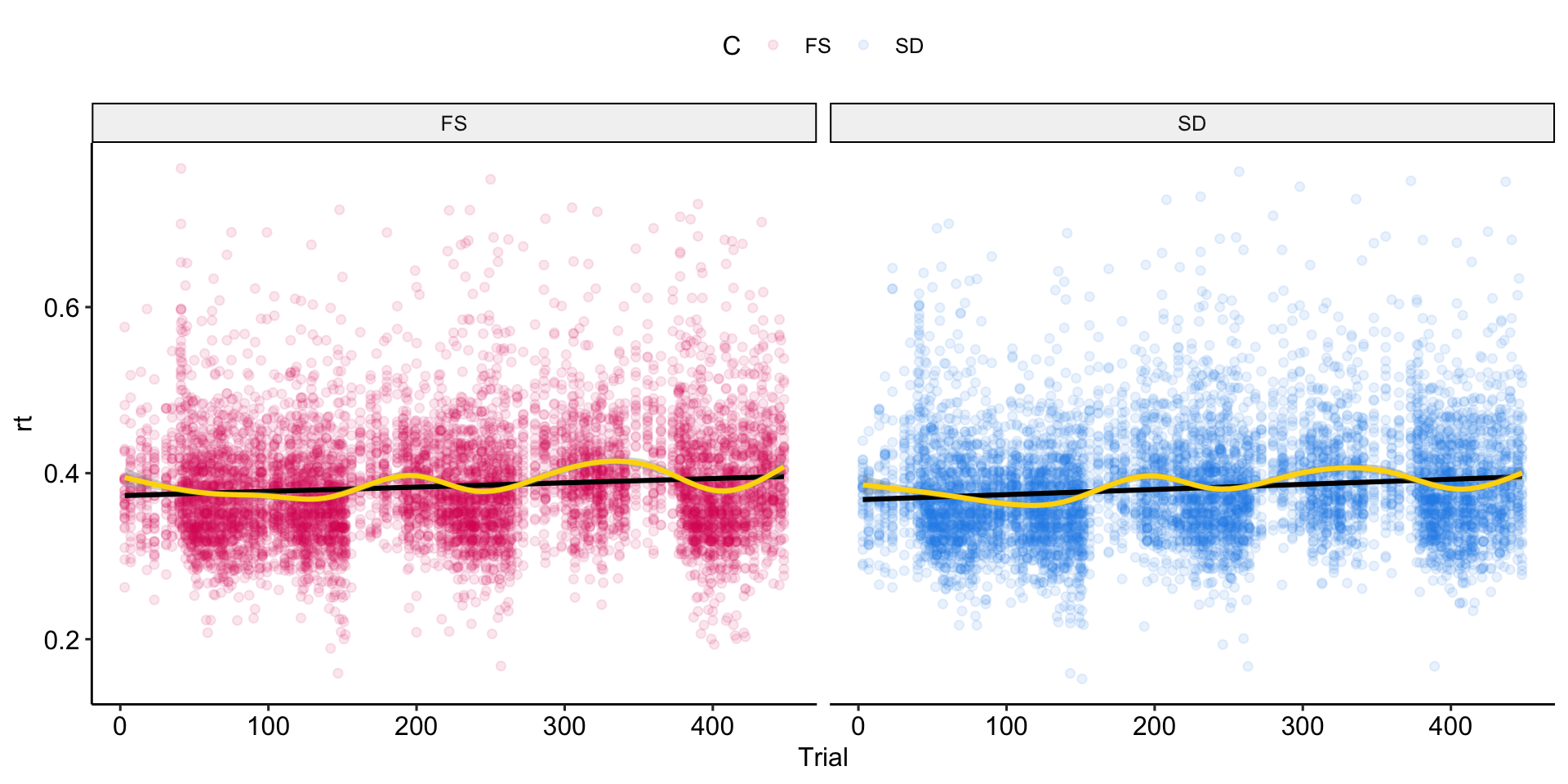
dat_clean2 %>% subset(target == "go.png" & rt > .15) %>% 
  ggplot(aes(y= rt, x = Trial, color = C))+
  geom_point(alpha = .1)+facet_wrap(~ C) +
  scale_color_manual(values = my_pal$pal1)+
  geom_smooth(method = "lm", color = "black", alpha = .5)+ #linear
   geom_smooth(method = "gam", #additive
              color = "gold")
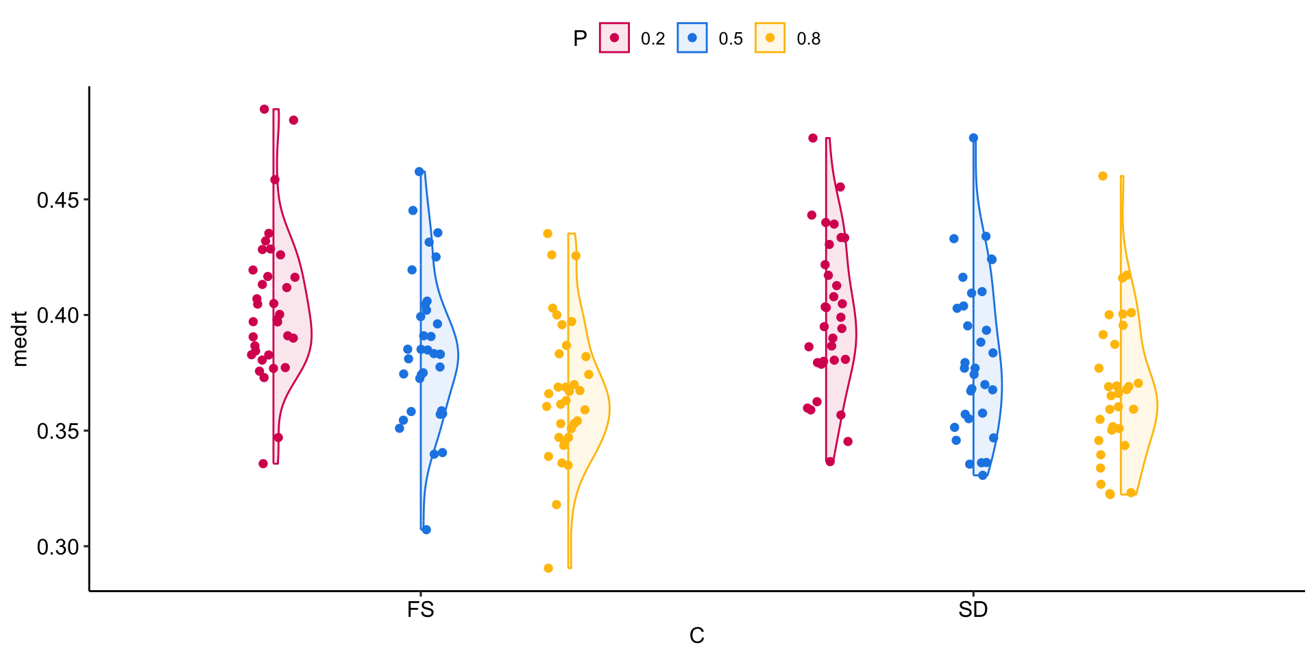
dat_clean2 %>% subset(target == "go.png" & rt > .15) %>% 
  group_by(id,C,P)%>%
  summarise(medrt = median(rt))%>%
  ggplot(aes(y= medrt, x = C, color = P, fill = P))+
  see::geom_violinhalf(position = position_dodge(width = .8),
                       alpha = .1)+
  geom_jitter(position = position_jitterdodge(jitter.width = .2,
                                              dodge.width = 0.8))+
  scale_color_manual(values = my_pal$pal1)+
  scale_fill_manual(values = my_pal$pal1)
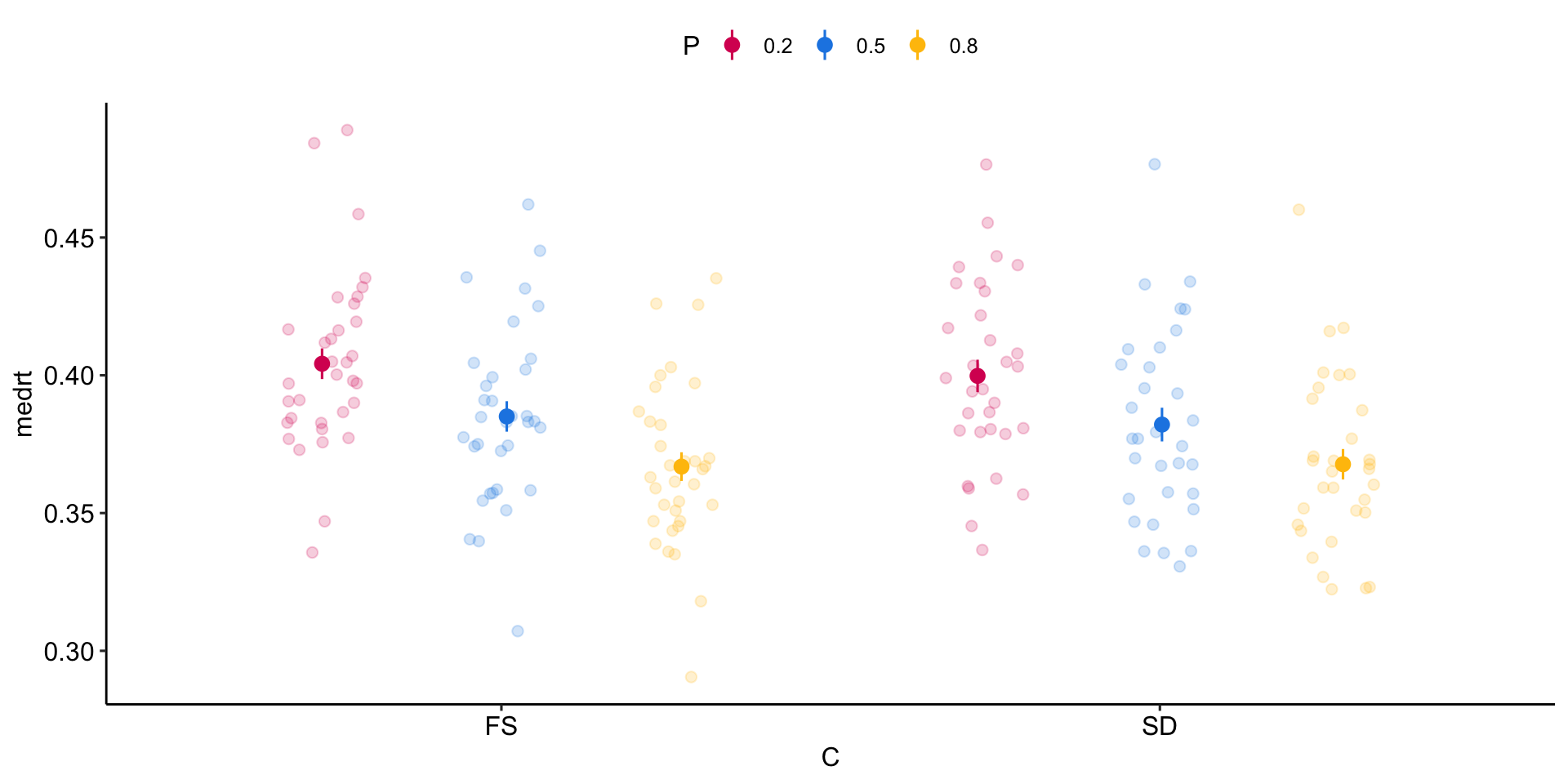
dat_clean2 %>% subset(target == "go.png" & rt > .15) %>% 
  group_by(id,C,P)%>%
  summarise(medrt = median(rt))%>%
  ggplot(aes(y= medrt, x = C, color = P, fill = P))+
  geom_jitter(alpha = .2, size = 2, position = position_jitterdodge(jitter.width = .3,
                                              dodge.width = 0.8))+
  stat_summary(size = .5, position =position_jitterdodge(jitter.width = .1,
                                              dodge.width = 0.8))+
  scale_color_manual(values = my_pal$pal1)+
  scale_fill_manual(values = my_pal$pal1)
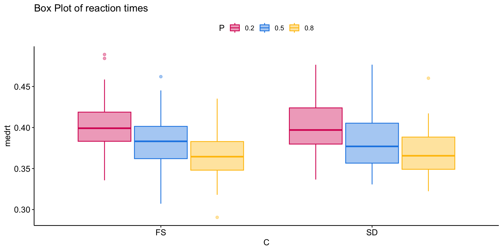
dat_clean2 %>% subset(target == "go.png" & rt > .15) %>% 
  group_by(id,C,P)%>%
  summarise(medrt = median(rt))%>%
  ggplot(aes(y= medrt, x = C, color = P, fill = P))+
  geom_boxplot(alpha = .4, position = position_dodge(width = .8))+
  scale_color_manual(values = my_pal$pal1)+
  scale_fill_manual(values = my_pal$pal1)+
  ggtitle("Box Plot of reaction times")
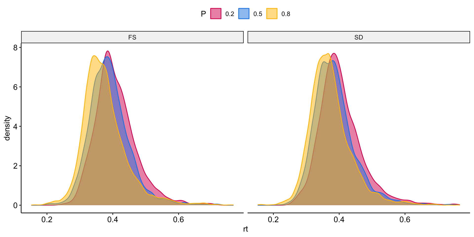
dat_clean2 %>% subset(target == "go.png" & rt > .15) %>% 
  ggplot(aes(x= rt,  color = P, fill = P))+
  geom_density(alpha = .5) +facet_wrap(~C)+
  scale_color_manual(values = my_pal$pal1)+
  scale_fill_manual(values = my_pal$pal1)

Saving plots

  1. Create an object containing your plot
  2. Save it
my_plot <- dat_clean2 %>% subset(target == "go.png" & rt > .15) %>% 
  ggplot(aes(x= rt,  color = P, fill = P))+ geom_density(alpha = .5) +
  facet_wrap(~C)+ scale_color_manual(values = my_pal$pal1)+
  scale_fill_manual(values = my_pal$pal1)+
  xlab("RTs in sec")

# create the plot folder
dir.create("plot")

# save inside the plot folder
ggsave("plot/my_plot.jpg", my_plot,dpi = 600, width = 18, 
       height = 10, units = "cm")

Tables

Another thing you may find useful is creating tables with, for example, descriptive statistics or the output of a statistical model. For these operations the flextable or kableExtra packages are very useful:

library(flextable);library(kableExtra)
descr <- dat_clean2%>%
  group_by(P,C)%>%
  summarise(medRT = round(median(rt, 
                                 na.rm = T),4),
            meanRT = round(mean(rt, 
                                na.rm = T),4),
            sd = round(sd(rt, na.rm = T),4))
descr
# A tibble: 6 × 5
# Groups:   P [3]
  P     C     medRT meanRT     sd
  <fct> <fct> <dbl>  <dbl>  <dbl>
1 0.2   FS    0.396  0.405 0.0659
2 0.2   SD    0.392  0.401 0.0728
3 0.5   FS    0.384  0.388 0.0634
4 0.5   SD    0.378  0.385 0.0639
5 0.8   FS    0.366  0.374 0.0679
6 0.8   SD    0.366  0.372 0.0646

Tables

tab <- descr |>
    flextable() |>
    theme_vanilla() |>
    autofit() |>
    colformat_double(digits = 3)
tab

P

C

medRT

meanRT

sd

0.2

FS

0.396

0.405

0.066

0.2

SD

0.392

0.401

0.073

0.5

FS

0.384

0.389

0.063

0.5

SD

0.378

0.385

0.064

0.8

FS

0.366

0.374

0.068

0.8

SD

0.366

0.372

0.065

Saving to a Word file

doc <- officer::read_docx() # Create an empty Word document

doc <- body_add_flextable(doc, value = tab) # Add the flextable

print(doc, target = "tabella.docx") # Save the file