Iterative programming

Example: if I ask you to use the print() function to write “hello world” in the console 5 times, how would you do it?

msg <- "hello world"
print(msg)

[1] "hello world"

print(msg)

[1] "hello world"

print(msg)

[1] "hello world"

print(msg)

[1] "hello world"

print(msg)

[1] "hello world"

What we are missing is a way to repeat a given operation without actually repeating the code manually.

There are several constructs that let us repeat operations; the most used are:

The for loop
The while loop
The repeat loop
The *apply family

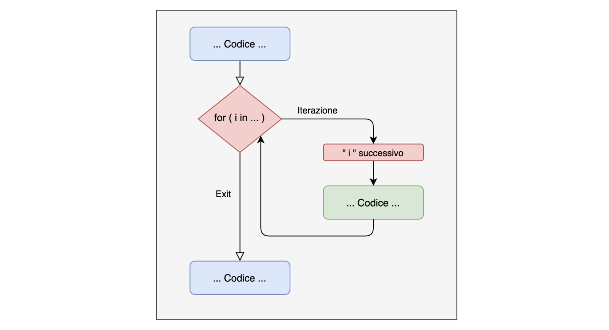
The `for` loop

The for loop is a structure that lets us repeat a portion of code a finite, pre-determined number of times.

A for loop is written as:

n <- 10
for(i in 1:n){
# which operations
}

If I want to print something 5 times, I can simply use a for loop:

for(i in 1:5){
print("hello world")
}

[1] "hello world"
[1] "hello world"
[1] "hello world"
[1] "hello world"
[1] "hello world"

Breaking down the `for` loop

for(){ }: this is the implementation in R (similar to the if statement)
i: this is called the iterator or index. It is a generic index that can take any value and name. By convention it is called i, j etc. It keeps track of the number of iterations our loop has to do
in <values>: this indicates the values the iterator will take inside the loop
{ # operations }: these are the operations the loop must perform

for(i in 1:5){
print(paste("hello world", i, sep = " "))
}

[1] "hello world 1"
[1] "hello world 2"
[1] "hello world 3"
[1] "hello world 4"
[1] "hello world 5"

The power of the for loop lies in the fact that the iterator i takes the values of the vector specified after in, one at a time:

for(i in 1:10){
  print(i)
}

[1] 1
[1] 2
[1] 3
[1] 4
[1] 5
[1] 6
[1] 7
[1] 8
[1] 9
[1] 10

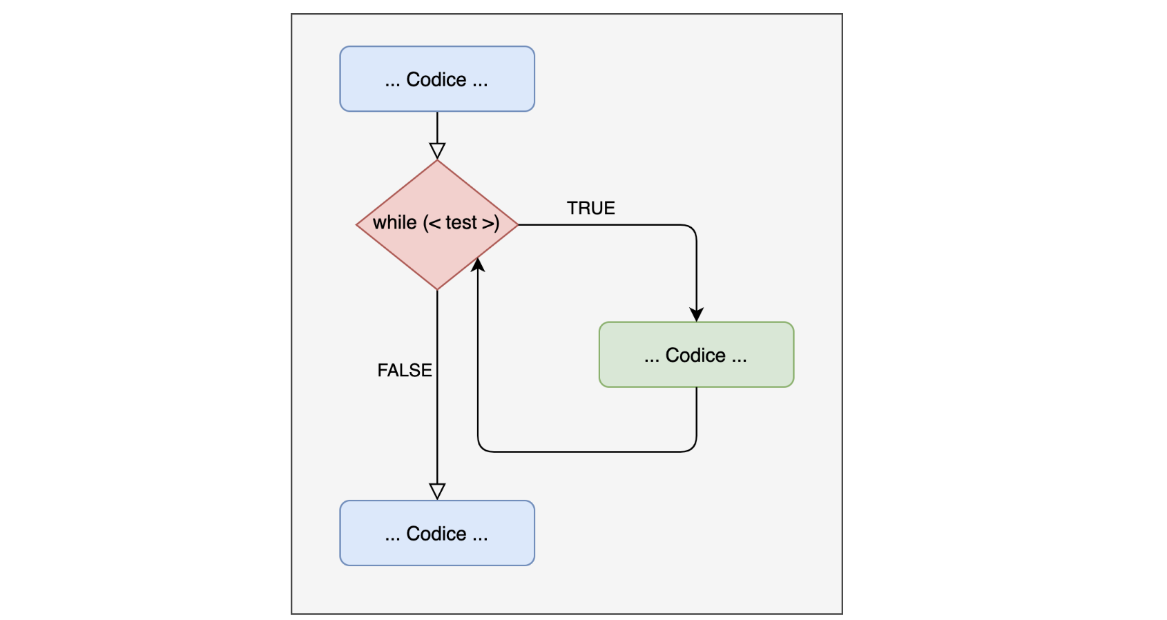
`For` with an index vs without

i represents the index of the elements of the vector vec

vec <- c(1,3,5,8)

for(i in 1:length(vec)){
  
  print(paste(i, vec[i], sep = " "))

  }

[1] "1 1"
[1] "2 3"
[1] "3 5"
[1] "4 8"

i directly represents each element of the vector vec

vec <- c(1,3,5,8)

for(i in vec){

  print(i)

}

[1] 1
[1] 3
[1] 5
[1] 8

The `while` loop

The while loop uses a logical condition instead of an iterator and a range of values as in the for loop. The loop keeps going as long as the condition is TRUE:

Try writing this while loop, see what happens and understand why

x <- 10

while (x < 15) {

  print(x)

}

The while loop is not pre-determined, so it always needs a way to be stopped, by making the condition false.

x <- 5

while (x < 15) {
  print(x)
  x <- x + 1
}

[1] 5
[1] 6
[1] 7
[1] 8
[1] 9
[1] 10
[1] 11
[1] 12
[1] 13
[1] 14

The `repeat` loop

The logic of the repeat loop is very similar to that of the while loop, but with 3 important differences:

it always performs at least one iteration
it emphasizes repetition until a condition is met
it uses the break command to stop

The `repeat` loop

Roll the die until a 6 comes up:

repeat{
  die_roll <- sample(1:6, 1)
  print(die_roll)
  if(die_roll == 6) break
}

[1] 2
[1] 5
[1] 3
[1] 3
[1] 1
[1] 5
[1] 3
[1] 4
[1] 2
[1] 2
[1] 3
[1] 5
[1] 4
[1] 4
[1] 6

`repeat` vs. `while`

repeat evaluates the condition at the end of the iteration, while while does it at the beginning. If the condition is not TRUE at the start, while does not run, whereas repeat does:

i <- 1
repeat {
  print(i)
  i <- i+1
  if(i > 3)break
  }

[1] 1
[1] 2
[1] 3

i <- 1
while (i < 4) {
  print(i)
  i <- i+1
  }

[1] 1
[1] 2
[1] 3

Example: the `sum()` function

Imagine we did not have the sum() function and wanted to recreate it: how would we do it? Any ideas?

Sum as iteration

Let’s break the sum down conceptually; we add up the numbers from 1 to 10:

I take the first one and add it to the second (total = 1 + 2)
I take the total and add it to the 3rd element: total = total + 3 …

In practice we have:

our vector to sum
a total object that progressively accumulates the previous sums

Sum as iteration

total <- 0 # initialize the total to 0
x <- 1:10 # vector x

for(i in 1:length(x)){ # for the whole length of x = 1:10
  total <- total + x[i]
}

Let’s put everything inside a function (i.e., I create a function that replicates what the sum function does)

my_sum <- function(x){
  total <- 0 # initialize the total to 0
  for(i in 1:length(x)){  # equivalent to 1:length(x)
    total <- total + x[i]
    }
  return(total)
}

x <- rnorm(100, mean = 0, sd = 1)

my_sum(x)

[1] 12.67144

sum(x)

[1] 12.67144

Iteration, applications

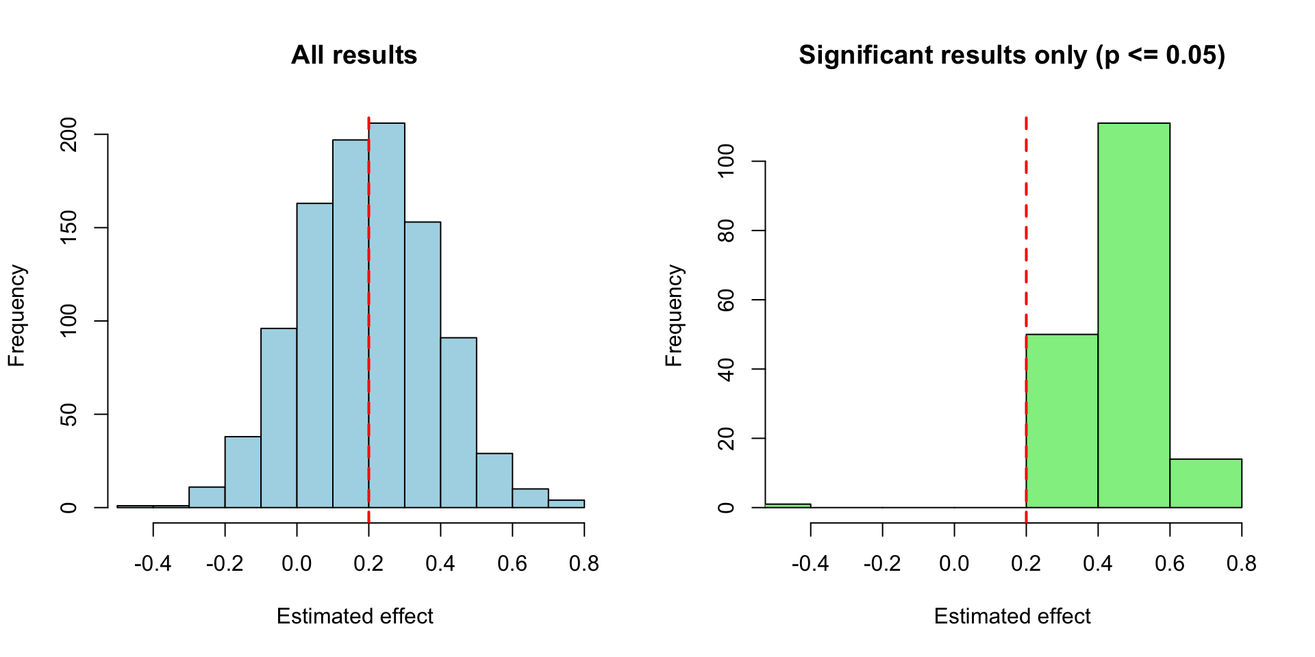
The for loop is also useful, for example, to simulate data and perfom a power analysis. Suppose we have a variable y (income) that depends on age:

Load the dataset:

mydf <- read.csv(file = "data/mydf_2.csv") # load the dataset

str(mydf)

'data.frame':   30 obs. of  4 variables:
 $ id     : int  1 2 3 4 5 6 7 8 9 10 ...
 $ age    : int  36 29 37 49 33 50 16 24 48 46 ...
 $ age_cat: chr  "adult" "young" "adult" "adult" ...
 $ age_z  : num  0.27244 -0.35627 0.36226 1.44004 0.00299 ...

Simulate the variable y (income) assuming it depends on age_z (age), so we need to extract age_z and choose an effect size

# Observed data
age_z <- mydf$age_z
eff_age <- .2 # age effect
nobs <- nrow(mydf)

Now the for loop …

set.seed(111) # for reproducibility
#initialize the empity vectors
niter <- 1000 # number of iterations
res_all <- rep(NA, niter)    # all estimated effects
p_val <- rep(NA, niter)      # all p-values

for(i in 1:niter) {
  
  y <- rnorm(nobs, mean = 0 + eff_age * age_z, sd = 1) 

  # linear model
  mod <- lm(y ~ 1 + age_z)

  # extract the effect estimate
  res_all[i] <- coef(mod)[2]

  # p-value of age_z
  p_val[i] <- summary(mod)$coefficients[2, 4]
}

Result:

# Keep only significant results
res_sig <- res_all[p_val <= 0.05]

# Descriptive statistics
cat("Proportion significant = Power:", mean(p_val <= 0.05), "\n")

Proportion significant = Power: 0.176

cat("Mean of all effects:", mean(res_all), "\n")

Mean of all effects: 0.1963144

cat("Mean of significant effects:", mean(res_sig), "\n")

Mean of significant effects: 0.450603

Nested `for` loops

Once you understand the iterative structure, you can easily extend it by putting a loop inside another one:

for(i in 1:3){ # level 1
  for(j in 1:3){ # level 2
      print(paste(i, j))
    }
}

[1] "1 1"
[1] "1 2"
[1] "1 3"
[1] "2 1"
[1] "2 2"
[1] "2 3"
[1] "3 1"
[1] "3 2"
[1] "3 3"

Two groups, Control and Treatment, with 3 participants each: a nested loop goes through every participant of every group.

groups <- c("Control", "Treatment")
for (group in groups) {     # outer loop: groups
  for (subj in 1:3) {       # inner loop: participants
    print(paste("Group:", group, "- Participant:", subj))
  }
}

[1] "Group: Control - Participant: 1"
[1] "Group: Control - Participant: 2"
[1] "Group: Control - Participant: 3"
[1] "Group: Treatment - Participant: 1"
[1] "Group: Treatment - Participant: 2"
[1] "Group: Treatment - Participant: 3"

For each group, the inner loop runs completely: 2 x 3 = 6 repetitions.

Now let’s simulate a reaction time (in ms) for each participant, and save it in a matrix: one row for each participant, one column for each group.

rt <- data.frame(Control = c(NA,NA, NA),
                 Treatment = c(NA,NA, NA))   # empty df
rt

  Control Treatment
1      NA        NA
2      NA        NA
3      NA        NA

The two indices of the loops are the row (i) and the column (j) of the cell to fill: rt[i, j]

set.seed(42)           # reproducibility
means <- c(500, 450)   # Control, Treatment

for (j in 1:2) {       # columns: groups
  for (i in 1:3) {     # rows: participants
    rt[i, j] <- round(rnorm(1, mean = means[j], sd = 50))
  }
}

rt

  Control Treatment
1     569       482
2     472       470
3     518       445

colMeans(rt)           # mean RT of each group

  Control Treatment 
 519.6667  465.6667

Now let’s practice!

Open this link and keep it open:

https://etherpad.wikimedia.org/p/arca-corsoR

Iterative programming