[1] 5Conditional programming
Programming in R
We will look at the main programming constructs and how they are applied in R. Many of the concepts presented are general, so they also apply to other programming languages. Here we will cover the most basic aspects; for more advanced applications we suggest the book: Advanced R
Topics
Programming constructs
Conditional programming
Iterative programming
Functions
Just like mathematical functions, a function in programming abstracts a series of operations (in our case a portion of code): given some inputs, it performs a series of operations and returns some outputs.
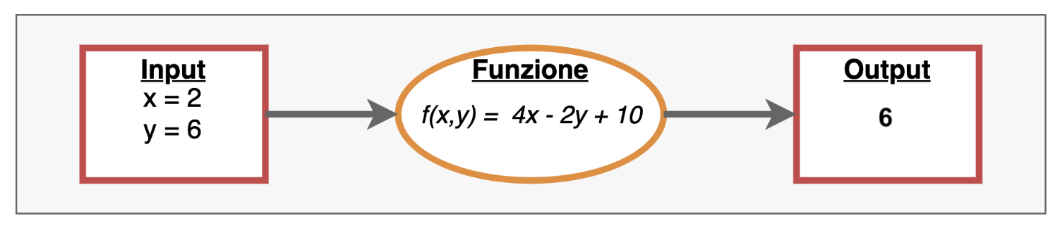
Functions - Creation
The command used to create a function in R is function(), followed by a pair of curly braces { } inside which we write the body of the function:
The function I created takes x and y as input, adds them, and returns the result as output.
Functions - Creation
We can perform many different operations inside a single function. It is better to use the return() command to explicitly define the output we want, for example…
Functions - Creation
Let’s take a repetitive operation often performed in data analysis: standardizing a variable (transforming it into z scores), i.e. subtracting its mean \(\mu_x\) from a vector x of observations and then dividing by the standard deviation \(\sigma_x\) :
\[ x_z = \frac{x - \mu_x}{\sigma_x} \]
Functions - Creation
To create this function we need to define:
arguments: variables to be defined (if not already defined)
body: the operations the function must perform using the arguments
output: what the function must return as a result
Functions - Creation
Arguments
The arguments are the variable parts of the function that are defined and then needed to run the function itself. In our function the only argument is the input vector. Just like mean and sd, we can add a second argument indicating whether to remove NAs:
Functions - Creation
Body
The body of the function contains the operations to perform using the input arguments. In our case we need to subtract the mean and divide by the standard deviation.
Functions - Creation
Output
The output is the result the function returns after performing all the operations. In our case we want the function to return the vector transformed into z scores. As we saw before, we can use the return() function, which explicitly tells the function what to return:
Functions - Creation
We have now created this function, which becomes an object in our environment, and we can use it
Functions - tips
- Curly braces
{}can be omitted if the code is all on the same line return()can be omitted if the last line is the desired output
Conditional programming - if
In programming we usually need not only to perform a series of operations BUT to perform operations depending on some conditions.
Conditional programming - if
The concept of if condition then do operation is translated in programming through what are called if statements

if statement
Let’s see an example
if statement - STOP
There is a family of functions with the is. prefix that returns TRUE when the object type matches the requested one and FALSE otherwise.
[1] 5.5Error in `myfun_stop()`:
! the vector must be numericif statement - STOP
There is a family of functions with the is. prefix that returns TRUE when the object type matches the requested one and FALSE otherwise.
if...else
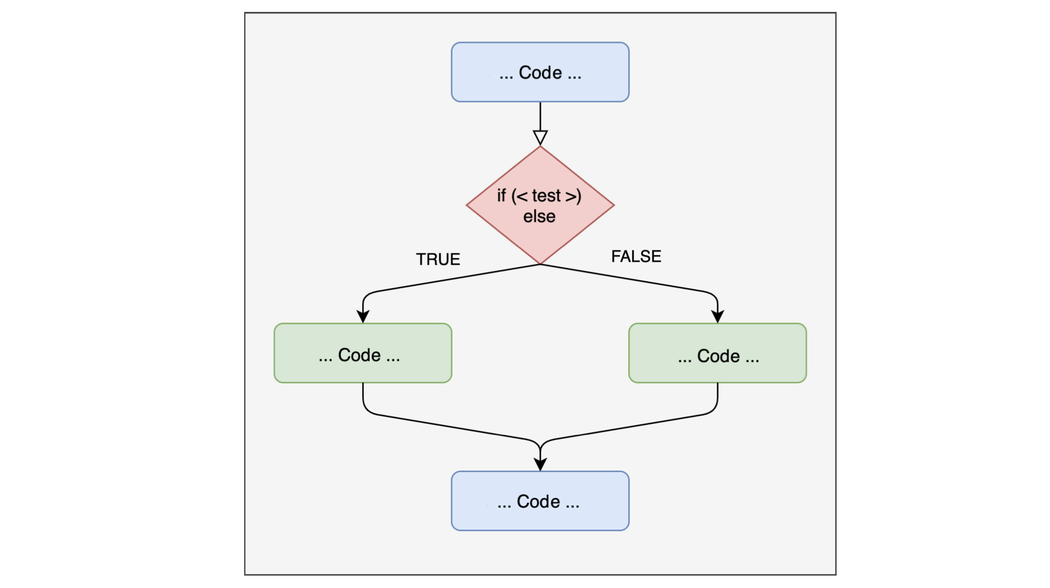
Using a single if may not be enough in some situations. Above all because we can see the if as a temporary detour from the main script that is taken only if a condition is true; otherwise the script goes on.
if...else
If we want a more “symmetric” structure, we can perform some operations if the condition is true (if) and others for all the other scenarios (else).
if...else
Let’s see an example
if...else
if...else - nested
if...else - nested
Conditional programming
To understand which conditional structure to use, it is important to understand the problem we need to solve well. Let’s take an example: imagine we have 2 types of data in R, strings and numbers. In this case it is enough to have an if statement that checks whether the element is a string/number and performs a given operation.
Conditional programming
Let’s write a function that returns the mean when the vector is numeric, and the frequency table otherwise.
Conditional programming
Let’s test the function
Conditional programming
One limitation of if statements is that they only work on a single value (i.e. they are not vectorized). So, while the my_summary function works because it evaluates whether the whole vector is numeric (is.numeric())…
Conditional programming
If we wanted to use the myfun_if function …
function (x)
{
    if (x > 0) {
        cat("The value is greater than 0\n")
    }
    cat("End of function")
}
<bytecode: 0x1454cf348>
it would not work…
Conditional programming
The vectorized version is obtained with the ifelse() function, whose arguments are the condition to test, the output if the condition is TRUE, and the output if it is FALSE
Conditional programming
When we need to test several alternatives we can create nested ifelse(). Imagine we have an age vector and want to create another vector where age is divided into 3 groups: child, adult, elderly:
[1] 60 45 68 64 57 24 19 69 43 20 [1] "elderly" "adult" "elderly" "elderly" "adult" "adult" "adult"
[8] "elderly" "adult" "adult" dplyr::case_when
When there are many conditions to test (roughly > 3), writing many nested ifelse() can be tedious. We can then use the dplyr::case_when() function from the dplyr package, which is a generalization of ifelse():
the results are identical…
dplyr::case_when
Recoding the values of a variable, for example reversing the items of a questionnaire, is easily done with dplyr::case_when():
[1] 2 2 4 3 4 2 3 5 3 5 3 2 5 4 5 1 1 1 1 3dplyr::case_when
These functions can also be applied to the variables in a dataframe:
# create a dataframe with id and age variables
mydf <- data.frame(id = factor(1:30), age = sample(14:50, 30))
# save it for later
readr::write_csv(mydf, file = "data/mydf.csv")
# create a third variable with "adolescent", "young", "adult"
mydf$age_cat <- factor(case_when(mydf$age > 30 ~ "adult",
                                 mydf$age <= 30 & mydf$age >= 20 ~ "young",
                                 mydf$age < 20 ~ "adolescent",
                                 TRUE ~ "error" # check for coding errors
                                    ))
str(mydf)
'data.frame': 30 obs. of 3 variables:
$ id : Factor w/ 30 levels "1","2","3","4",..: 1 2 3 4 5 6 7 8 9 10 ...
$ age : int 36 29 37 49 33 50 16 24 48 46 ...
$ age_cat: Factor w/ 3 levels "adolescent","adult",..: 2 3 2 2 2 2 1 3 2 2 ...Importing a function
We have already seen that the library() command loads a package, making the functions it contains available. Without needing to create a package, we can still organize our own functions effectively.
Importing a function
We have two options
write the functions in the same script where they are used
write a separate script and import all the functions it contains
Importing a function
Here too it is a matter of style and convenience; in general:
if we have many functions, it is better to write them in one or more separate files and then import them at the beginning of the main script
if we have few functions, we can keep them in the main script, perhaps in a dedicated section at the beginning
Importing a function
In the second case it is enough to write the function, and it will be saved as an object in the main environment. For the first scenario, we can use the source("utl/script.R") function:
Importing and using a function
Now my functions are available as objects in my environment and I can use them:
'data.frame':   30 obs. of  2 variables:
 $ id : num  1 2 3 4 5 6 7 8 9 10 ...
$ age: num 36 29 37 49 33 50 16 24 48 46 ... id age age_cat age_z
1 1 36 adult 0.272440521
2 2 29 young -0.356268374
3 3 37 adult 0.362256078
4 4 49 adult 1.440042755
5 5 33 adult 0.002993852
6 6 50 adult 1.529858312Now let’s practice!
Open this link and keep it open: