Introduction 2

Topics

Objects
- types of objects
- creating/naming an object
- data types
Operators
- mathematical
- relational
- logical

Objects

Everything we can create in R is called an object (e.g., numbers, vectors, matrices, functions).

number <- 4
number

[1] 4

my_vector <- c(1,2,3,4)
my_vector

[1] 1 2 3 4

my_matrix <- matrix(nrow = 2, ncol = 2, data = my_vector)
my_matrix

     [,1] [,2]
[1,]    1    3
[2,]    2    4

Functions

Everything we do in R is calling functions on objects. Functions allow us to create and modify objects.

my_vector

[1] 1 2 3 4

mean(x = my_vector)

[1] 2.5

my_vector_mean <- mean(my_vector)
my_vector_mean

[1] 2.5

Creating/naming objects

Objects are created with the assignment arrow <- or =

x1 <- 3 # name <- object
x1

[1] 3

x2 = 3 # name = object
x2

[1] 3

Rules for naming objects

A name must start with a letter and can contain letters, numbers, underscores ( _ ), or dots (.).
It may also start with a dot (.), but in that case it cannot be followed by a number.

.3 <- 3

Error in `0.3 <- 3`:
! invalid (do_set) left-hand side to assignment

.x <- 3

It must not contain special characters such as #, &, $, ?, etc.

It must not be a reserved word, i.e. one of the words used by R with a special meaning (?reserved).

function <- 3

Error in parse(text = input): <text>:1:10: unexpected assignment
1: function <-
             ^

TRUE <- 3

Error in `TRUE <- 3`:
! invalid (do_set) left-hand side to assignment

if <- 3

Error in parse(text = input): <text>:1:4: unexpected assignment
1: if <-
       ^

Some names are not forbidden but are discouraged

[1] TRUE

T == TRUE

[1] TRUE

T <- FALSE;

T == TRUE  #?????

[1] FALSE

T == FALSE #?????

[1] TRUE

Using “.” in object names (for example, “my.data”) is fine in R but is not allowed in Python, where “.” is part of the language syntax.

Across languages, the naming conventions for longer, multi-word variable names favour snake_case (for example, “my_data”) or camelCase (for example, “myData”), and abbreviations where appropriate (for example, “unipdData” rather than “university_of_padova_dataset”).

R is case-sensitive

Name <- "Margherita"
name <- "margherita"
Name == name

[1] FALSE

Name <- "margherita"
name <- "margherita"
Name == name

[1] TRUE

Where are objects stored?

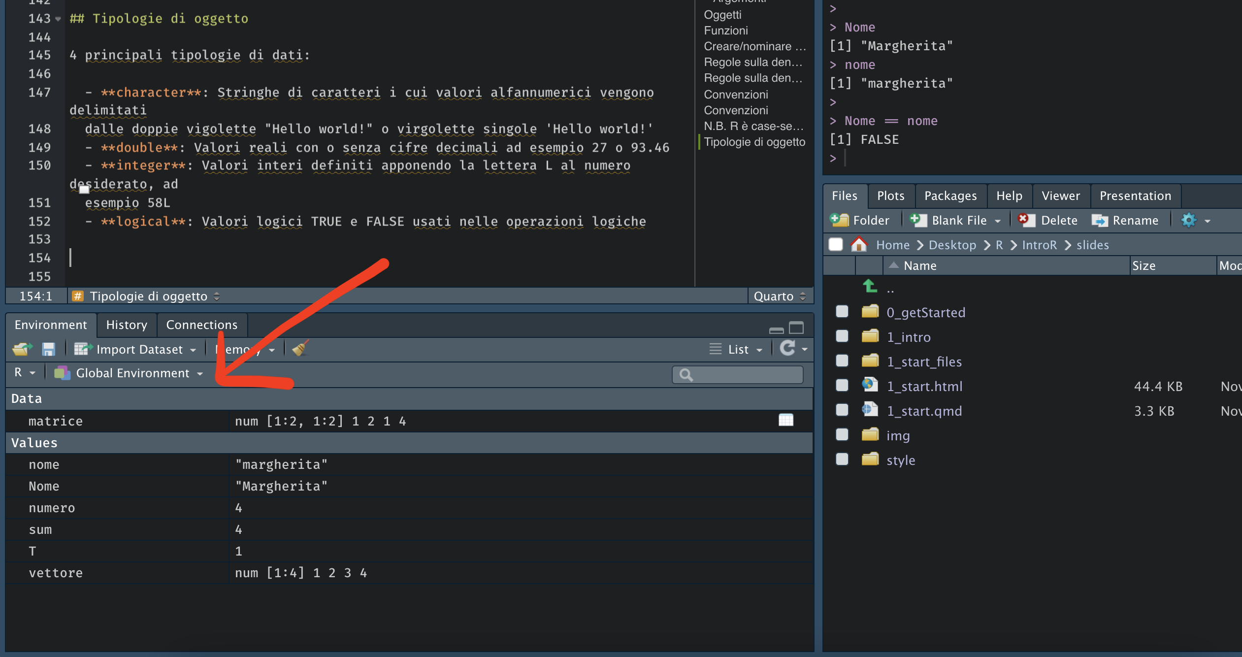
By default, objects are created in the global environment, which can be accessed with ls() or viewed in R Studio together with some additional information:

Removing objects

We can remove an object from our environment with the rm("objectname") command.

We can also completely clear/empty our environment with the rm(list = ls()) command.

Data types

character: Character strings whose alphanumeric values are delimited by double quotes “Hello world!” or single quotes ‘Hello world!’
numbers:
- double: Real values with or without decimal digits, for example 27 or 93.46
- integer: Integer values defined by appending the letter L to the number, for example 58L

Mathematical Operators

Function	What does it do?	Example	Result
`+`	addition	`5.4 + 6.1`	`11.5`
`-`	subtraction	`9 - 4.3`	`4.7`
`*`	multiplication	`7 * 1.4`	`9.8`
`/`	division	`9/3`	`3`
`%%`	remainder	`9%%2`	`1`
`^`	power	`15 ^ 2`	`225`

Mathematical Operators

Function	What does it do?	Example	Result
`abs`	absolute value	`abs(-8)`	`8`
`sqrt`	square root	`sqrt(225)`	`15`
`exp`	exponential function	`exp(0)`	`1`
`log`	natural logarithm	`log(1)`	`0`
`round`	rounding, integer	`round(1.738)`	`2`
`round`	rounding	`round(1.738, 2)`	`1.74`

Mathematical Operations

The order of operations in R follows the rules of mathematics.

Examples

# Without parentheses
1 + 2 * 3

[1] 7

# With parentheses
(1 + 2) * 3

[1] 9

Relational Operators

In R we can evaluate whether a given relation is true or false. R will evaluate the statement and return TRUE if the statement is true or FALSE if the statement is false.

Relational Operators

Function	Name	Example	Result
`==`	equal	`30 == 30`	`TRUE`
`!=`	not equal	`30 != 30`	`FALSE`
`>`/`>=`	greater/or equal	`30 > 10` `30 >= 10`	`TRUE` `TRUE`
`<`/`<=`	less/or equal	`30 < 10` `10 <= 10`	`FALSE` `TRUE`
`%in%`	inclusion	`10%in%c(1,2,10)`	`TRUE`

It doesn’t only work with numbers!

Name <- "Margherita"

name <- "margherita"

Name == name

[1] FALSE

NB. Remember that = is different from ==

Logical Operators

In R we can combine several relations to evaluate a given statement.

x <- 30 # Assign the value 30 to x.

Function	Name	Example	Result
`&`	Conjunction (AND)	`x>25 & x<60`	`TRUE`
`\|`	Inclusive disjunction (OR)	`x>25 \| x>60`	`TRUE`
`!`	Negation (NOT)	`!(x<18)`	`TRUE`

Logical Operators

x <- 30 # Assign the value 30 to x.
x

[1] 30

x>25 & x>60

[1] FALSE

x>25 | x>60

[1] TRUE

!(x>18)

[1] FALSE

TRUE is equivalent to 1 and FALSE to 0

TRUE == 1

[1] TRUE

TRUE == 2

[1] FALSE

FALSE == 0

[1] TRUE

FALSE == 1

[1] FALSE

TRUE is equivalent to 1 and FALSE to 0

I create an example vector containing the words home (repeated 3 times) and shop (repeated 2 times):

example <- c("home", "home", "home","shop", "shop") #?rep
example

[1] "home" "home" "home" "shop" "shop"

# Which words in `example` are equal to home?
example == "home"

[1]  TRUE  TRUE  TRUE FALSE FALSE

sum(example == "home") # why?

[1] 3

Order of Evaluation

When evaluating whether statements are true, R performs the operations in the following order:

Mathematical operators (e.g., ^, *, /, +, -, etc.)
Relational operators (e.g., <, >, <=, >=, ==, !=)
Logical operators (e.g., !, &, |)

If in doubt about the order in which operations are executed, the best thing to do is to use round brackets ( ) to remove any possible ambiguity.

Let’s practice!

Open this link and keep it open: https://etherpad.wikimedia.org/p/arca-corsoR